As we have seen, when they converge, power series are very well behaved. But Fourier (trigonometric) series were not at all well behaved. That was a puzzle which made them a lightning rod for mathematical study in the nineteenth century.
For example, consider the question of uniqueness. We saw in Chapter 7 that if a function could be represented by a power series, then that series must be the Taylor series. More precisely, if
Using the techniques that he employed to solve the heat flow problem (see Chapter 5), Fourier showed that if a “general” function \(f(x)\) defined on the interval \([0,1]\) could be expressed as a trigonometric series
If \(\sum_{m=0}^\infty \left[ a_n\cos(2n \pi x) + b_n\sin (2n\pi
x)\right] \) converges uniformly to \(f\) on \([0, 1]\text{,}\) then Fourier’s term–by–term integration is perfectly legitimate and the coefficients will be as given above.
However we have seen that the convergence of a Fourier series need not be uniform. So term–by–term integration of a Fourier series is not guaranteed to produce the integral of the associated function.
Such considerations led to a generalization of the integral by Henri Lebesgue in \(1905\text{.}\) Lebesgue’s profound work settled the question: “Is a bounded pointwise converging trigonometric series the Fourier series of a function?” We will (very briefly) describe some of Lebesgue’s work in Section 12.3.
But before we can do that we will need to understand the pioneering work of Georg Cantor (1845–1918) on Set Theory in the late 19th century. Cantor’s work was profound, had far reaching implications in modern mathematics, and leads to some seemingly very weird conclusions.
We ask: If these two series are equal must it be true that \(a_n=a^\prime_n\) and \(b_n=b^\prime_n\text{?}\) We can reformulate this uniqueness question as follows: Suppose
Intuitively, it certainly seems reasonable to suppose so, but at this point we have enough experience with infinite sums to know that we need to be very careful about relying on the intuition we have gained from finite sums.
Answering this question led Cantor to study the makeup of the real number system. This in turn opened the door to the twentieth century view of mathematics. In particular, Cantor proved the following result in \(1871\) ([8], p. 305).
In his attempts to nail down precisely which “certain values” could be exceptional Cantor was led to examine the nature of subsets of real numbers and ultimately to give a precise definition of the concept of infinite sets and to define an arithmetic of “infinite numbers.”
Observe that this is not a trivial generalization. Although the exceptional points are constrained to be finite in number, this number could still be extraordinarily large. That is, even if the series given above differed from zero on \(10^{\left(10^{100000}\right)}\) distinct points in the interval \(\left(0, 10^{-\left(10^{100000}\right)}\right)\) the coefficients still vanish. This remains true even if at each of these \(10^{\left(10^{100000}\right)}\) points the series converges to \(10^{\left(10^{100000}\right)}\text{.}\) This is truly remarkable when you think of it this way.
At this point Cantor became more interested in these exceptional points than in the Fourier series problem that he’d started with. The next task he set for himself was to see just how general the set of exceptional points could be. Following Cantor’s lead we make the following definitions.
Let \(S\subseteq \RR\) and let \(a\) be a real number. We say that \(a\) is a limit point (or an accumulation point) of \(S\) if there is a sequence \((a_n)\) with \(a_n\in S-\left\{a\right\}\) which converges to \(a\text{.}\)
Let \(S\subseteq\RR\) and let \(a\) be a real number. Prove that \(a\) is a limit point of \(S\) if and only if for every \(\eps>0\) the intersection of the interval \((a-\eps, a+\eps)\) with \(S\) contains more than the single point \({a}\text{.}\)
Let \(S\subseteq\RR\text{.}\) The set of all limit points of \(S\) is called the derived set of \(S\text{.}\) The derived set is denoted \(S^{\prime}\text{.}\)
Don’t confuse the derived set of a set with the derivative of a function. They are completely different objects despite the similarity of both the language and notation. The only thing that they have in common is that they were somehow “derived” from something else.
The notion of the derived set forms the foundation of Cantor’s exceptional set of values. Specifically, let \(S\) again be a set of real numbers and consider the following sequence of sets:
Cantor’s work was instrumental in the re–examination of the foundations of mathematics whereby mathematical ideas were recast in the language of sets at the turn of the twentieth century. Nowadays we do this naturally, so it doesn’t seem profound, but recasting mathematics in terms of Set Theory has fundamentally shaped our modern approach. We’ve already seen this in Definition 12.0.5, Problem 12.0.6, and Definition 12.0.7 where we recast Cantor’s definition of a limit point into set theoretic terms.
It turns out that we can also rewrite concepts such as limits and continuity in terms of sets. This led to a subject known as point set topology. Presenting all of topology would require an entire new course with an entire new book, so we will only give a brief glimpse at how analysis concepts can be recast in set theoretic form.
Recall that a closed interval is one which contains its endpoints. Similarly, a set of real numbers \(S\) (not necessarily an interval) is called closed if it contains all of its limit points. A closed interval is also a closed set as the next problem shows.
The converse of Problem 12.1.1 is not true. That is, not every closed set is also a closed interval. Convince yourself that each of the sets below is closed.
At this point you’ve probably guessed that the definition of an open set can be modeled on the definition of open interval. That is true, but Definition 12.1.3 is easier to use.
Again, we could spend an entire course exploring these concepts, but for our introduction we will only show how the concept of continuity can be repackaged into a statement involving sets. To keep things simple we will restrict our attention to functions \(f(x)\) whose domain \(D\) is an open set of real numbers. The following notation will be helpful.
Show that \(f(x)\) is continuous at \(x=a\) if and only if for every open set \(V\) containing \(f(a)\) there is an open set \(U\) containing \(a\) with \(f(U)\subset
V\text{.}\)
Problem12.1.9.Topological Definition of Continuity.
Show that a function \(f(x)\) is continuous on a set \(D\subset \RR \) if and only if for every open set of real numbers \(V\subseteq \RR \text{,}\) the preimage of \(V\) is open.
The value of the reformulation of continuity seen in Problem 12.1.9 in terms of open sets (and similar definitions involving limits) is that it allows the concept of continuity to be generalized beyond the realm of real numbers to sets where the distance between points is either irrelevant or is simply not meaningful.
Given an arbitrary nonempty set \(S\text{,}\) we define a topology on \(S\) to be a collection \(\tau\text{,}\) of subsets of \(S\) (which we designate to be the open sets) which satisfy the following conditions.
\(S\) and \(\emptyset \) must be in \(\tau \text{.}\)
This relatively simple idea generalizes our notion of open intervals in the real numbers and can be applied to a wide range of sets. We won’t go into this very deeply, but we note that if we have a function \(f:S\to T\) from one topological space into another, we can define a continuous function to be one where the preimage of any open set in the topology on \(T\) must be open in the topology on \(S\text{.}\) It would be hard to overstate the impact of generalizaions of this sort on modern mathematics.
Cantor’s work with Fourier series prompted him to study the sizes of various infinite sets. The following theorem follows directly from our previous work with the NIP and will be very handy later. It is a slightly weaker version of the NIP which says that the intersection of a sequence of nested closed intervals will be non–empty even if their lengths do not converge to zero.
By Corollary 9.4.5 of Chapter 9, we know that a bounded increasing sequence such as \((x_n)\) converges, say to \(c\text{.}\) Since \(x_n\leq x_m\leq y_n\) for \(m>n\) and \(\limit{m}{\infty}{x_m}=c\text{,}\) then for any fixed \(n\text{,}\)\(x_n\leq c\leq y_n\text{.}\) This says \(c\in\left[x_n,
y_n\right]\) for all \(n\in\NN\text{.}\)
Suppose \(\limit{n}{\infty}{\abs{y_n-x_n}}>0\text{.}\) Show that there are at least two points, \(c\) and \(d\text{,}\) such that \(c\in[x_n, y_n]\) and \(d\in[x_n, y_n]\) for all \(n\in\NN\text{.}\)
Our next theorem says that in a certain, very technical sense there are more real numbers than there are counting numbers [5]. This probably does not seem terribly significant. After all, there are plenty of real numbers which are not counting numbers. But what makes this startling is that the same cannot be said about all sets which strictly contain the counting numbers. Some such sets are even the same “size” as the counting numbers in a sense that we will make precise in this section.
For the sake of obtaining a contradiction assume that the sequence \(S\) contains every real number; that is, \(S=\RR\text{.}\) As usual we will build a sequence of nested intervals \(\left(\left[x_i,
y_i\right]\right)_{i=1}^\infty\text{.}\)
Let \(x_1\) be the smaller of the first two distinct elements of \(S\text{,}\) let \(y_1\) be the larger and take \(\left[x_1,y_1\right]\) to be the first interval.
Next we assume that \(\left[x_{n-1}, y_{n-1}\right]\) has been constructed and build \(\left[x_n, y_n\right]\) as follows. Observe that there are infinitely many elements of \(S\) in \(\left(x_{n-1}, y_{n-1}\right)\) since \(S=\RR\text{.}\) Let \(x_n\) and \(y_n\) be the first two distinct elements of \(S\) such that
So, suppose that \(c=s_p\) for some \(p\in\NN\text{.}\) Then only \(\left\{s_1, s_2,\ldots, s_{p-1}\right\}\) appear before \(s_p\) in the sequence \(S\text{.}\) Since each \(x_n\) is taken from \(S\) it follows that only finitely many elements of the sequence \((x_n)\) appear before \(s_p=c\) in the sequence as well.
Let \(x_l\) be the last element of \((x_n)\) which appears before \(c=s_p\) in the sequence and consider \(x_{l+1}\text{.}\) The way it was constructed, \(x_{l+1}\) was one of the first two distinct terms in the sequence \(S\) strictly between \(x_l\) and \(y_l\text{,}\) the other being \(y_{l+1}\text{.}\) Since \(x_{l+1}\) does not appear before \(c=s_p\) in the sequence and \(x_l\lt c\lt
y_l\text{,}\) it follows that either \(c=x_{l+1}\) or \(c=y_{l+1}\text{.}\) However, this gives us a contradiction as we know from formula (12.2.1) that \(x_{l+1}\lt c\lt y_{l+1}\text{.}\)
So how does this theorem show that there are “more” real numbers than counting numbers? Before we address that question we need to be very careful about the meaning of the word “more” when we’re talking about infinite sets.
How do we know that \(B\) is the bigger set? One way is to simply count the number of elements in both sets. Clearly \(B\) is bigger since \(\abs{A}=4\) and \(\abs{B}=5\) and \(4\lt 5\text{.}\) But we have no way of counting the number of elements of an infinite set. Indeed, it isn’t even clear what the phrase “the number of elements” might mean when applied to an infinite set. So we need to find another way.
When we count the number of elements in a finite set we are matching up the elements of the set with a set of consecutive positive integers, starting at \(1\text{.}\) Thus since
it is clear that the elements of \(B\) and the set \(\left\{1,2,3,4,5\right\}\) can be matched up as well. And it doesn’t matter what order either set is in. They both have \(5\) elements.
Such a match–up is called a one–to–one correspondence. In general, if two sets can be put in one–to–one correspondence then they are the same “size.” Of course the word “size” has lots of connotations that will begin to get in the way when we talk about infinite sets, so instead we will say that the two sets have the same cardinality. Speaking loosely, this just means that they are the same size. Speaking very loosely it means that they have the same “number” of elements.
Speaking precisely, if a given set \(S\) can be put in one–to–one correspondence with a finite set of consecutive integers beginning at \(1\text{,}\) say \(\left\{1,2,3,\ldots, N\right\}\text{,}\) then we say that the cardinality of the set is \(N\) because both sets have the same cardinality. It is this notion of one–to–one correspondence, along with the next two definitions, which will allow us to compare the sizes (cardinalities) of infinite sets.
Any set which can be put into one–to–one correspondence with \(\NN=\left\{1,2,3,\ldots\right\}\) is called a countably infinite set. Any set which is either finite or countably infinite is said to be countable.
Since \(\NN\) is an infinite set, we have no symbol to designate its cardinality so we have to invent one. The symbol used by Cantor and adopted by mathematicians ever since is \(\aleph_0\text{.}\) Thus the cardinality of any countably infinite set is \(\aleph_0\text{.}\)
With these two definitions in place we can see that Theorem 12.2.3 is nothing more nor less than the statement that \(\RR\) is not countably infinite, for if it were then a one–to–one correspondence with \(\NN \) would enable the entire set \(\RR\) to be written as a sequence, violating Theorem 12.2.3.
In Problem 12.2.7 we saw several examples where the union of finitely many countably infinite sets yields another set which is also countably infinite. But what about a countably infinite union of countably infinite sets? Surely that will yield an uncountably infinite set.
All of our efforts to build an uncountable set from a countable one have come to nothing. In fact many sets that at first “feel” like they should be uncountable are not. This makes the uncountability of \(\RR\) all the more remarkable.
The failure is in the methods we’ve used so far. It is possible to build an uncountable set using just two symbols if we’re clever enough. Give some thought to how this might be done. We will return to this question in Section 12.4.
Let \((a,b)\) and \((c,d)\) be two open intervals of real numbers. Show that these two sets have the same cardinality by constructing a one–to–one onto function between them.
Theorem 11.2.1 states that if (Riemann) integrable functions \(f_n\) converge uniformly to an integrable function \(f\) on \([a,b]\) then limit evaluation and integration are commutative operations:
Thus we can integrate a power series term–by–term because as we saw in Theorem 11.3.9 all power series converge uniformly on any closed interval \([-b,b]\) contained inside their intervals of convergence, \((-r,
r)\text{.}\) However the converse of Theorem 11.2.1 is not true.
In fact Problem 11.1.8 is an example of a function which is the pointwise limit of continuous functions where integration and limit evaluation commute. We did not comment on it at the time because we weren’t prepared to talk about integration yet. Now we are.
Notice that for any partition \(P\) the lower sum \(L\left(P\right)=0\text{,}\) so the lower Darboux integral is \(0\text{.}\) To find the upper Darboux integral, let \(0\lt \eps \lt 1\) and use the partition \(P=\left\{ 0, 1-\eps,
1\right\} \) to show that the upper Darboux integral is less than or equal to \(\eps
\text{.}\) Be sure to explain how the conclusion follows from this observation.
As a result of Problem 12.3.2 we have one example of a pointwise limit where integration and limit evaluation commute, thus affirming that uniform convergence is not a necessary condition. A natural question to ask at this point is, “What is necessary?” In other words, can we find weaker conditions on the convergence that still allow commutativity? The next problem begins to address — but does not fully answer — that question.
Extend your result in part (a) to show that the integral of \(f\) is unchanged if there are finitely many discontinuities: \(\left\{c_k\right\}_{k=1}^n \text{.}\)
Let \(f\) be a bounded function on \([a,b]\text{.}\) Do you think the integral of \(f\) will remain unchanged when the set of discontinuities is countably infinite? Explain.
You do not yet know enough about infinite sets to answer this question definitively, so we are not asking you to prove anything. Just explain what your intuition is telling you. There is no right or wrong answer yet. But there will be when we revisit this question in Problem 12.3.31.
\begin{align*}
P_n(x) = x^n, \amp{}\amp{}\text{ and }
\amp{}\amp{} \Upsilon_n(x)= \begin{cases}n\amp \text{ if } x\in\left(0,\frac{1}{n}\right)\\ 0\amp \text{ otherwise } \end{cases}.
\end{align*}
We know from Problem 12.3.2 that for the sequence \(\left(
P_n(x)\right)_{n-1}^\infty
\text{,}\) we can commute integration and limit evaluation. But by Problem 11.2.3 we cannot do this for the sequence \(\left( \Upsilon_n(x)\right)_{n-1}^\infty
\text{.}\) What do you suppose is the difference between the two?
Assume \(\left(f_n\left(x\right)\right)\) is a sequence of Riemann–integrable functions which converges pointwise to a Riemann integrable function \(f(x)\) on \([a,b]\text{.}\) Assume also that this sequence is uniformly bounded, namely, that there is a real number \(B\) with \(\abs{f_n\left(x\right)}\le B,\ \)for all \(x\in
[a,b]\) and for all \(n\text{.}\) Then
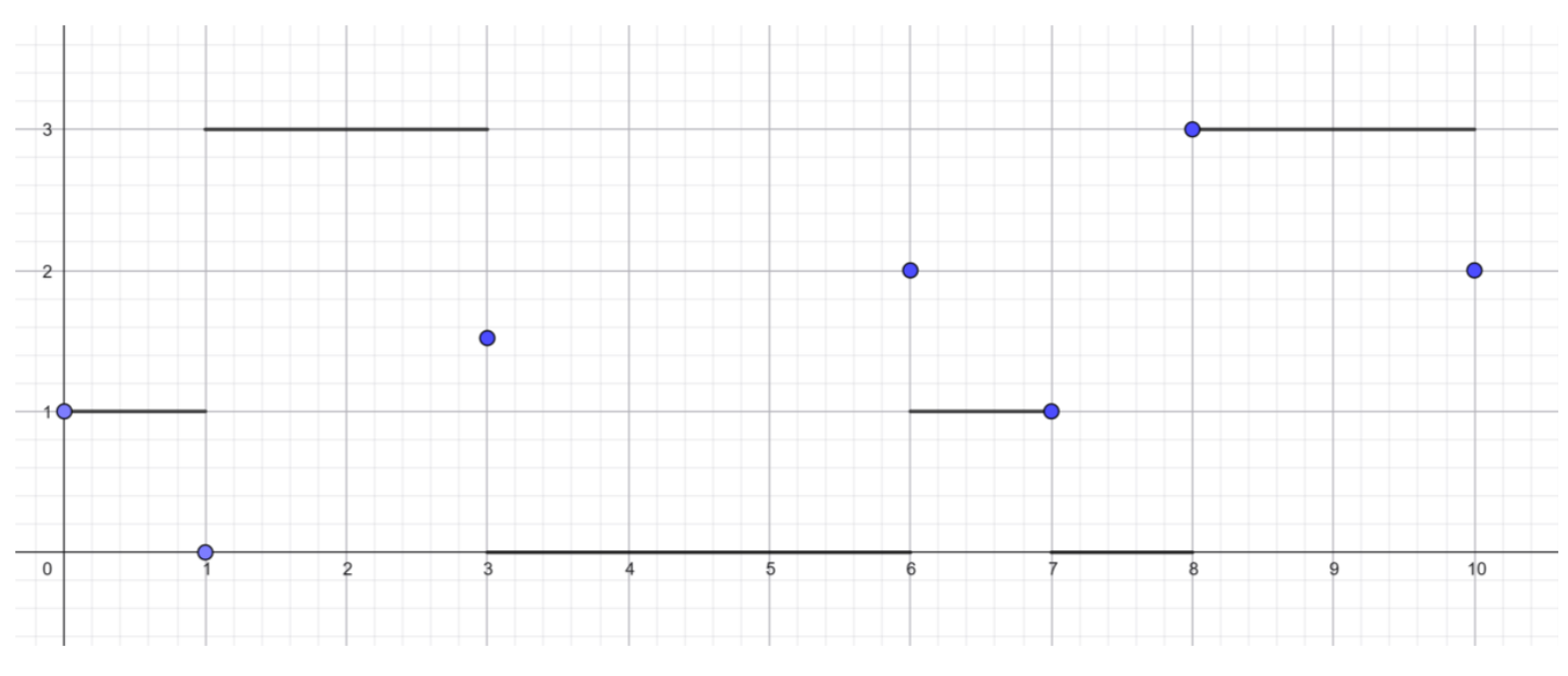
It is not necessarily true that the limit function \(f\) in Arzelà’s Bounded Convergence Theorem will be automatically Riemann integrable. To see this consider the following example.
From Problem 12.3.3 we see that each \(f_n\) is Riemann integrable. Show that the sequence\(\left(f_n\right)_{n=1}^\infty \) converges pointwise to the Dirichlet Function
\begin{equation*}
D\left(x\right)=
\begin{cases}
1
\amp{} \text{if } x \text{ is rational} \\
0 \amp{} \text{if } x \text{ is irrational}
\end{cases}
\end{equation*}
which is not Riemann integrable as we saw in Problem 10.4.10.
We will not provide a direct analytic proof of Arzelà’s Bounded Convergence Theorem. Instead we will show that it is a special case of a more general result.
Earlier in this chapter we saw how the concepts of continuity and the limit could be restated in terms of sets and set theory. Set theory also played a role in generalizing the notion of an integral. As we said before, the story of integration is complex with many entry points. To provide a full accounting would take another course (and another book) so we will provide only a glimpse into this story and see how it relates to the swapping of limits and integrals. In what follows many of the details will be glossed over in favor of a larger view.
As an entry point into this world, consider the Dirichlet Function again. Recall from Problem 10.4.10 that the Dirichlet Function
\begin{equation*}
D(x)=
\begin{cases}
0, \amp \text{ if } x \text{ is irrational}\\
1, \amp \text{ if } x \text{ is rational}
\end{cases}
\end{equation*}
is not Riemann (Cauchy, Darboux) integrable. Dirichlet invented his function as an example of a non–integrable function. For our purposes it has no importance beyond that. However the existence of non–(Riemann)integrable functions suggests the question: Can the integral be defined in such a way as to capture all of the intuitive features of (Riemann) integration known to \(18\)th century mathematicians and which also allows us to integrate something as seemingly bizarre as the Dirichlet Function?
Cantor’s work on the cardinality of infinite sets provides some insight. A countable set like \(\QQ \) is smaller than an uncountable set (in the sense that there is no one–to–one correspondence between them), but we haven’t yet tried to express how much smaller because we didn’t have any way to measure the size of either set in order to compare their sizes numerically.
Despite being infinite, countable sets are small in a sense we will make clear shortly. But uncountable sets are altogether different. They can be as small as a countable set or as large as all of the real numbers, depending on how they are built. We will explore this further in Problem 12.3.33.
In the same way that the value of a function on a finite number of points in its domain does not affect its Riemann integral (see Problem 12.3.3) it seems, intuitively at least, that the values a function takes on a countably infinite piece of its domain should not affect the value of its integral either. We need a way to measure the size of sets, particularly infinite sets, which clearly displays that a countable set is small among the infinite sets.
In order to extend integration beyond the Riemann integral Henri Lebesgue (1875–1941) devised such a measure His ideas were later generalized leading to the area of mathematics called measure theory. Lebesgue is not the only mathematician to address the problem of defining a measure for sets. But he was one of the first and his ideas have become foundational so we will focus on the Lebesgue measure and the Lebesgue integral.
\(\mu{}\) is translation invariant. More precisely, if \(S \) is a subset of \(\RR \text{,}\)\(x\) is any real number, and \(S_x=\left\{s+x\left| s\in S
\right.\right\} \) then
The purpose of the first and third statements in Definition 12.3.11 should be clear. Since we are looking to generalize the concept of length the measure of an interval should be its length, which does not depend on its position. For example,
The conditions in Definition 12.3.11 are clearly modeled on the properties of the length of an interval. The reason for formalizing it is that we want measure other kinds of sets in \(\RR{}\text{.}\) For example using this definition we can compute \(\mu (\ZZ )\text{,}\)\(\mu (\NN{}) \) and \(\mu (\QQ)
\text{.}\) What would you guess each of these will be?
Actually defining such a measure is more delicate than it might appear to be as we will see. But this is enough to serve our immediate purposes. We will focus on what Lebesgue introduced in his \(1902\) doctoral dissertation Intégrale, longueur, aire (Integral, length, area) which is now known as Lebesgue Measure.
Suppose \(\cal{C}\) is a collection of open intervals in \(\RR\) and let \(S\) be any set in \(\RR\text{.}\) Then \(\cal{C}\) is called an open cover of \(S\) if and only if every element of \(S\) is contained in at least one of the open sets in \(\cal{C}\text{.}\) If \(\cal{C}\) contains only finitely many open sets then \(\cal{C}\) is called a finite open cover of \(S\text{.}\)
Loosely speaking, an open cover of a set \(S\) is a collection of open intervals which “cover” \(S\) (hence the name). Obviously every open interval is an open cover of itself.
Let \(S\subset\RR \) and let \(C\) be the collection of all countable open covers \(\left\{ (a_n, b_n) \left| n=1, 2, 3,
\ldots{}\right.\right\} \) of \(S\text{.}\) The outer measure of \(S\) is given by
That we called \(\mu_o (S)\) an outer measure suggests that there might be something called an inner measure and indeed there is. It’s definition is given in Definition 12.3.16.
The names of the inner and outer measures are descriptive. To compute \(\mu _o\) we consider a set of numbers generated by a collection of sets which contain \(S\text{.}\) To compute \(\mu_i\) we consider a set of numbers generated by a collection of sets which are contained within \(S\text{.}\) When these are the same we have the Lebesgue Measure.
All seems pretty straightforward at this point, but here is where one of the difficulties lies: For a given set, there is no guarantee that the inner and outer measures must be equal. When they are not the set is said to be non–measurable. The first non–measurable set was described by Giuseppe Vitali (1875-1932) in \(1905\text{.}\) Creating such a set requires the use of something called the Axiom of Choice and careful study of Set Theory. We will see how complicated sets can be in the next section.
From a practical point of view, almost every set you encounter will likely be (Lebesgue) measurable. In summary, the collection of measurable sets has the following properties.
Every interval \(I\subset \RR\) is measurable and \(\mu
\left(I\right)\) is equal to the length of \(I\text{.}\)
For the remainder of this section we will only be discussing and using the Outer Measure. This will be enough to give you a good intuitive feel for the Lebesgue Integral which we define below. We have included the definitions of Inner Measure and Lebesgue Measure for completeness.
Let \(S=\{s_1, s_2, s_3, \dots \}\) be countably infinite set of real numbers. Let \(\eps \gt 0\) be given. There is a collection of open intervals \((a_n,\
b_n)\) with
Observe that Definition 12.3.17 does not say that anything is equal to zero. Explain how we can still conclude in Theorem 12.3.19 that the set \(S\) has measure zero.
Despite the existence of non–measurable sets of real numbers, Lebesgue was able to generalize the idea of a Riemann integral in a meaningful way. Here is an overall look at his ideas.
Speaking very loosely, if we want to compute \(\int_a^bf(x)\dx{x} \) where \(f(x)\ge 0\) using the Riemann (Cauchy) integral we partition the \(x-\)axis into adjacent intervals with width \(\dx{x}\) and then construct (infinitesimal) rectangles with area \(f(x)\cdot{}\dx{x}\) from each differential. Summing these areas (computing \(\int_a^b f(x)\dx{x}\)) provides the value of the definite integral.
Lebesgue’s idea was to find all rectangles with a common height first, gather them together, and sum those areas. In letter to a colleague he described his process as follows:
“I have to pay a certain sum, which I have collected in my pocket. I take the bills and coins out of my pocket and give them to the creditor in the order I find them until I have reached the total sum. This is the Riemann integral. But I can proceed differently. After I have taken all the money out of my pocket I order the bills and coins according to identical values and then I pay the several heaps one after the other to the creditor. This is my integral.”
\begin{equation*}
D\left(x\right)=
\begin{cases}
1 \amp{} \text{ if } x \text{ is rational} \\
0 \amp{} \text{ if } x \text{ is irrational}
\end{cases}
\end{equation*}
is a simple function on \(\left[0,1\right]\text{.}\)
In order to define the Lebesgue integral of a more general function we proceed much as we did in Section 10.4 where we defined the upper and lower Darboux integrals in Subsection 10.4.2.
Definition12.3.25.Upper and Lower Lebesgue Integrals.
Suppose \(f\) is a bounded function defined on a measurable set \(E\) with \(\mu \left(E\right)\lt{}\infty \text{.}\) We define the upper and lower Lebesgue integrals, respectively, by
Just as with the upper and lower Darboux integrals (Problem 10.4.7), we want to show that \(I_*\le I^*\text{.}\) We’ll do this in part (b) of Problem 12.3.27. In preparation we’ll first show that for any simple functions, \(s(x)\) and \(t(x)\) defined on \(E\) with \(s\left(x\right)\le t(x)\) for all \(x\in E\text{,}\) we have
Note that if \(S=S_1\cup S_2\) and \(S_1\cap
S_2=\emptyset \text{,}\) then \({\chi }_S={\chi }_{S_1}+{\chi
}_{S_2}\text{.}\) This can be extended to more than two sets, namely if \(S=\bigcup^n_{j=1}{S_j}\) where \(S_j\) are pairwise disjoint, then
where \(E_j=s^{-1}\left(\left\{a_j\right\}\right)\text{.}\) Note that with this notation, \(E=\bigcup^n_{j=1}{E_j}\) where \(E_j\) are pairwise disjoint. Next suppose we have two simple functions \(s\left(x\right)\le t(x)\) defined on a measurable set \(E\) with \(\mu \left(E\right)\lt{}\infty \text{.}\) Using the notation we developed, we can write these simple functions as
\begin{align*}
s(x)=\sum^n_{j=1}a_j\chi_{E_j}(x)\amp{}\amp{}
\text{ and }
\amp{}\amp{} t\left(x\right)=\sum^m_{i=1}b_i{\chi
}_{F_i}\left(x\right).
\end{align*}
where \(\displaystyle{}E=\bigcup_{j=1}^nE_j = \bigcup_{i=1}^mF_i \text{.}\) Notice that for each \(j\text{,}\) we can write
Use the above ideas to show that if \(s\left(x\right),\ t(x)\) are two simple functions defined on a measurable set \(E\) with \(\mu
\left(E\right)\lt\infty \) with \(s\left(x\right)\le t(x)\text{,}\) then
We say that \(f\) is Lebesgue integrable on a measurable set \(E\text{,}\) provided that the Upper and Lower Lebesgue Integrals are equal: \(I^*=I_*\text{.}\)
Any bounded function which is Riemann (Darboux) integrable on a finite interval \([a,b]\) is automatically Lebesgue integrable and the values of the integrals are the same. The reason for this is straightforward: An upper Darboux sum \(U(P)\) is the integral of a simple function greater than or equal to \(f\) and a lower Darboux sum \(L(P)\) is the Lebesgue integral of a simple function less than or equal to \(f\text{.}\)
Use the result in part (a) to explain why a bounded function which is Riemann (Darboux) integrable must also be Lebesgue integrable and the values of the integrals are equal.
The Lebesgue Integral is more general than the Riemann Integral in the sense that there are functions which are Lebesgue but not Riemann integrable. We’ve already seen the Dirichlet function but there are others. The Lebesgue integral also shares the typical properties of a Riemann integral: integral of a sum equals sum of the integrals, the Fundamental Theorem Of Calculus, etc.
There is also a precise characterization for when a function is Lebesgue integrable. In a sense, Lebesgue consolidated a number of ideas and results about integration dating literally back to ancient times into a holistic approach by taking full advantage of results from modern Set Theory. As an example of this, we will examine, without proof, two of Lebesgue’s more important results.
Notice that we have avoided the question of the integrability of a function with uncountably many discontinuities. That is because it is the measure of the set, not its cardinality, which determines its integrability properties. And there are uncountable sets with both zero and non–zero measure. Perhaps the most famous of the former is Cantor’s middle–third set.
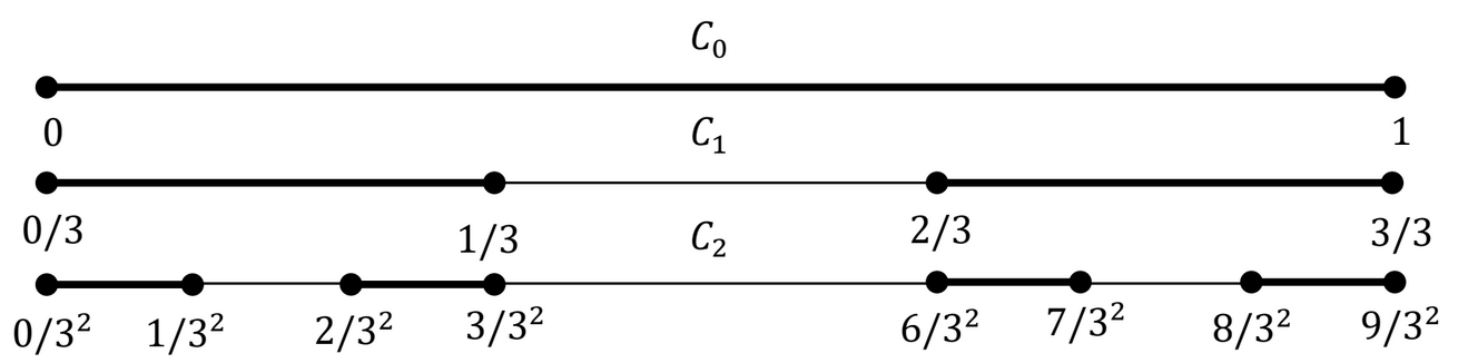
Loosely speaking, the Cantor middle–third set is constructed iteratively by deleting the “middle–third” of the interval \([0,1]\text{,}\) then deleting the “middle–third” of what is left, and continuing at each subsequent step to delete “middle–thirds” of what remains. More precisely, let \(C_0=[0,1]\) and define
and so on creating the sets \(C_0, C_1, C_2, C_3, \cdots
\text{.}\) The Cantor set is the intersection of all of these: \(C=\bigcap^{\infty }_{n=0}{C_n}\text{.}\)
Upon first considering Cantor’s middle–third set it seems intuitively clear that it consists entirely of the endpoints of the deleted intervals, which would make it a countable set (why?). Figure 12.3.32 certainly gives that impression, and if it were true then the Cantor set would have measure zero (why?).
But intuition is an unreliable tool and it must always be questioned. In fact, the Cantor set has the same cardinality as \(\RR\text{,}\) and yet its measure is zero as you will see in the next problem. We will return to the uncountabilty of the Cantor set in Problem 12.4.9.
Notice that in the first stage we remove an interval of length \(\frac{1}{3}\text{.}\) In the second stage, we remove two intervals of length \(\frac{1}{9}\) each. In the third stage, we remove four intervals of length \(\frac{1}{27}\) each. In the fourth stage we remove eight intervals of length \(\frac{1}{81}\) each. At each subsequent stage we removed twice as many intervals of length \(\frac{1}{3}\) that of the previous stage. Use this observation to show that \(\mu \left(\left[0, 1\right]-C\right)\) can be expressed as an infinite series whose sum is \(1\text{.}\)
Suppose \(E\) is a measurable set with \(\mu
\left(E\right)\lt{}\infty \) and \(\left(f_n\right)\) is a sequence of Lebesgue integrable functions on \(E\) which converges pointwise to \(f\) on \(E\) except possibly on a set \(M\) of measure 0. If there is a Lebesgue integrable function \(g\) such that \(\left|f_n\left(x\right)\right|\le g(x)\) for all \(x\in E-M\) and for all \(n\text{,}\) then \(f\) is Lebesgue integrable and
In the interest of conserving space we have presented a stripped down view of the modern development of integration theory, but the road from Riemann’s integral to Lebesgue’s was neither straight nor smooth. Cauchy, Riemann, Darboux and many others along the way developed their own ideas for a rigorous formulation of the integral concept.
If you are interested in learning more, you can begin by reading about Thomas Jan Stietles, Arnaud Denjoy, Oskar Perron, and Émile Borel, to name a few. You might also find the book [1] and the article [2] interesting. The latter describes an integral definition independently developed in the \(1960\)’s by Jaroslav Kurzwell and Ralph Henstock which is more general than the Lebesgue integral and is arguably easier to teach and understand.
After employing his ideas on infinite sets of real numbers to study trigonometric series, Cantor gravitated toward applying his ideas to sets in general. For example, once he showed that there were two types of infinity (countable and uncountable), the following question was natural, “Do all uncountable sets have the same cardinality?”
Just like not all “non–dogs” are cats, there is, a priori, no reason to believe that all uncountable sets should have the same cardinality. However constructing uncountable sets of different sizes is not as easy as it sounds.
For example, what about the line segment represented by the interval \([0,1]\) and the square represented by the set \([0,1]\times[0,1]=\left\{(x,y)\ |\ 0\leq x,y\leq
1\right\}\text{.}\) It certainly seems reasonable that set of points in a two dimensional square must be a larger infinite set than set of points in the one dimensional line segment. But Cantor was able to show that these two sets have the same cardinality. Remarkably, Cantor himself had trouble accepting this idea. In his \(1877\) correspondence of this result to his friend and fellow mathematician, Richard Dedekind, (1831–1915) he said, “I see it, but I don’t believe it!”
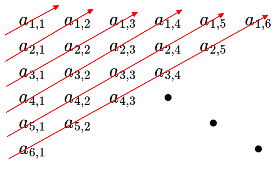
The following argument illustrates the idea of Cantor’s proof. We define the following function \(f:[0,1]\times[0,1]\rightarrow [0,1]\text{.}\) First, we represent the coordinates of any point \((x,y)\in [0,1]\times[0,1]\) by their decimal representations \(x=0.a_1 a_2 a_3\cdots\) and \(y=0.b_1 b_2 b_3\cdots\text{.}\) Even terminating decimals can be written this way as we could write \(0.5=0.5000\cdots\text{.}\) We can then define \(f(x,y)\) by
Consider the sequence \((0.9,0.99,0.999,\cdots)\text{.}\) Determine that this sequence converges and, in fact, it converges to \(1\text{.}\) This suggests that \(0.999\cdots=1\text{.}\)
Similarly, we have \(0.04999\cdots=0.05000\cdots\text{,}\) etc. To make the decimal representation of a real number in \([0,1]\) unique, we must make a consistent choice of writing a terminating decimal as one that ends in an infinite string of zeros or an infinite string of nines (with the one exception \(0=0.000\cdots\)).
Cantor was able to overcome this technicality and demonstrate a one–to–one correspondence, but rather than go into that we will simply assert that using either convention it is possible to show that the function \(f\) in equation (12.4.1) is one–to–one and onto. As a result the set \([0,1]\times[0,1]\) has the same cardinality as \([0,1]\) which is an uncountable subset of \(\RR\text{.}\)
Finally Cantor’s Theorem below is the tool we need to answer the question we began this section with: “Do all uncountable sets have the same cardinality?”
It is clear that \(S\) can be put into one–to–one correspondence with a subset of \(P(S)\) (why?), which means that \(P(S)\) is at least as large as \(S\) itself. In the finite case \(\abs{P(S)}\) is strictly greater than \(\abs{S}\) as the following problem shows. It also demonstrates why \(P(S)\) is called the power set of \(S\text{.}\)
Let \(S=\left\{a_1,a_2,\cdots,a_n\right\}\text{.}\) Consider the following correspondence between the elements of \(P(S)\) and the set \(T\) of all \(n\)-tuples of yes (Y) or no (N):
Assume for contradiction, that there is a one–to–one correspondence \(f:S\rightarrow P(S)\text{.}\) Consider \(A=\left\{x\in S\ |\ x\not\in f(x)\right\}\text{.}\) Since \(f\) is onto, then there is \(a\in A\) such that \(A=f(a)\text{.}\) Is \(a\in A\) or is \(a\not\in A?\)
In light of Cantor’s Theorem it is clear that there are sets which are larger (in the sense of Cantor) than \(\RR{}\text{.}\) Specifically \(\abs{P(\RR)}\gt \abs{\RR }\text{.}\)
Actually it turns out that \(\RR\) and \(P(\NN)\) have the same cardinality. This can be seen in a roundabout way using some of the ideas from Problem 12.4.4. Specifically, let \(T\) be the set of all sequences of zeros or ones.
The half–open interval \((0,1]\) has the same cardinality as \(\RR\) and we can show that it has the same cardinality as \(T\) as well by expressing them in binary form. Specifically every real number in \([0,1]\) can be written as
where \(a_j\in\left\{0,1\right\}\text{.}\) We have to account for the fact that binary representations such as \((0.0111\cdots)_2\) and \((0.1000\cdots)_2\) represent the same real number in a manner analagous to Problem 12.4.2 so we will impose the convention that no representations will end in an infinite string of zeros.
In that case we see that \((0,1]\) has the same cardinality as \(T-U\text{,}\) where \(U\) is the set of all sequences ending in an infinite string of zeros.
Problem 12.4.6 shows that \(U\) itself is a countable set so it follows that \(\RR\text{,}\)\(T-U\text{,}\)\(T\text{,}\) and \(P(N)\) all have the same cardinality. The following two problems show that deleting a countable set from an uncountable set does not change its cardinality.
Let \(Y=Y_0\text{.}\) Since \(X-Y_0\) is an infinite set, then by the previous problem it contains a countably infinite subset \(Y_1\text{.}\) Likewise since \(X-(Y_0\cup
Y_1)\) is infinite it also contains a countably infinite subset \(Y_2\text{.}\) Again, since \(X-(Y_0\cup Y_1\cup Y_2)\) is an infinite set then it contains a countably infinite subset \(Y_3\text{,}\) etc. For \(n=1, 2, 3,\cdots \text{,}\) let \(f_n:Y_{n-1}\rightarrow Y_n\) be a one–to–one correspondence and define \(f:X\rightarrow X-Y\) by
In the previous section, we mentioned that the Cantor middle–thirds set is uncountable. We will now prove that fact by showing that \(C\) contains a set which has the same cardinality as the set \(T\) of all sequences of zeros or ones, which is uncountable.
To see this, we will express the real numbers in \([0,1]\) in ternary (base three) form in a manner analogous to the binary representation seen in equation (12.4.2). That is, each number in \([0, 1]\) can be written in the form
but again this can be handled by simply choosing one representation or the other just as we did with both the binary and the decimal representations above. In what follows, we will adopt the convention that our ternary representations will not end in an infinite string of \(2\)’s. Since such representations form a countably infinite set (why?), it follows from Problem 12.4.7 and Problem 12.4.8 that the cardinality of the Cantor set is unaffected.
where \(a_2,a_3, \dots \in \{0,1,2\}\) (discarding infinite strings of \(2\)’s). In other words, \(C_1\) contains the set of all real numbers whose first ternary digit after the “ternary point” 1
The ternary point is for base \(3\) is just like the decimal point for base \(10\) representations.
is either \(0\) or \(2\text{.}\) By the same token
This says that \(C_2\) contains the set of all real numbers whose first two ternary digits are either \(0\) or \(2\) (discarding infinite strings of \(2\)’s). Similarly,
where \(a_4,a_5, \cdots \in \{0,1,2\}\) (discarding infinite strings of \(2\)’s), so that \(C_3\) contains the set of all real numbers whose first three ternary digits are either \(0\) or \(2\) (discarding infinite strings of \(2\)’s).
Continuing in this manner, we see that the Cantor set \(C=\bigcap^{\infty }_{n=0}{C_n}\) contains all the real numbers whose ternary expansions consist of \(0\) or \(2\text{.}\)
We observed in Section 12.3 that it seems intuitively clear that the Cantor set consists entirely of the endpoints of the intervals that are not removed at each step. But this set of endpoints is countable (why?) so in light of Problem 12.4.9 that can’t possibly be true. So the Cantor set must contain points that are not in the set of included endpoints.
According to our argument above the number \((0.020202\cdots )_3\) is in the Cantor set. Show that it is not the endpoint of any of the intervals used to construct the Cantor set.
As we indicated before, Cantor’s work on infinite sets had a profound impact on mathematics in the beginning of the twentieth century. For example, in examining the proof of Cantor’s Theorem, the eminent logician Bertrand Russell (1872–1970) devised his famous paradox in 1901.
Through the work of Cantor and others, sets were becoming a central object of study in mathematics. Mathematical concepts were being reformulated in terms of sets, as we saw in Section 12.1. The idea was that set theory was to be a unifying theme of mathematics but Russell’s paradox set the mathematical world on its ear because it showed that the naive understanding of a set as “just a collection of objects” leads to logical difficulties.
To have such a contradiction occurring at the most basic level of mathematics was scandalous. It forced a number of mathematicians and logicians to carefully devise the axioms by which sets could be constructed. To be honest, most mathematicians still approach set theory from a naive point of view as the sets we typically deal with are what we might characterize as “normal sets.” Such an approach is called Naive Set Theory (as opposed to Axiomatic Set Theory). Attempts to put set theory and logic on solid footing led to the modern study of symbolic logic and ultimately the design of computer (machine) logic.
Another place where Cantor’s work had a profound influence in modern logic comes from something we alluded to before. We showed before that the unit square \([0,1]\times [0,1]\) had the same cardinality as an uncountable subset of \(\RR\text{.}\) In fact, Cantor showed that the unit square had the same cardinality as \(\RR\) itself and was moved to advance the following in \(1878\text{.}\)
Cantor was unable to prove or disprove the Continuum Hypothesis conjecture (along with every other mathematician at the time). In fact, proving or disproving the Continuum Hypothesis, was one of David Hilbert’s famous 23 problems which he presented as a challenge for the mathematics community at the International Congress of Mathematicians in \(1900\text{.}\)
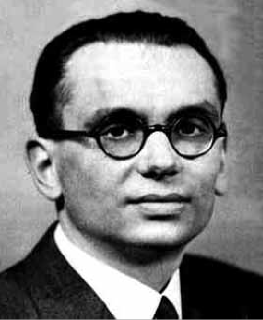
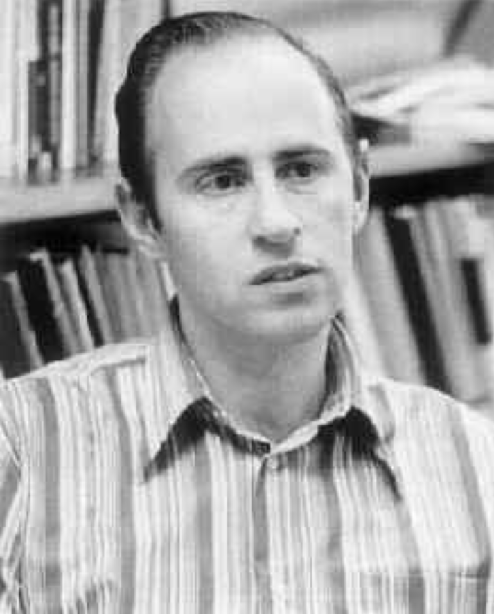
Efforts to prove or disprove Conjecture 12.4.15 were in vain and with good reason. In \(1940\text{,}\) the logician Kurt Gödel showed that the Continuum Hypothesis could not be disproved from the Zermelo-Fraenkel Axioms of set theory. In 1963, Paul Cohen (1934–2007) showed that the Continuum Hypothesis could not be proved using the Zermelo-Fraenkel Axioms, either. In other words, the Zermelo-Fraenkel Axioms do not contain enough information to decide the truth of the hypothesis.
We are willing to bet that at this point your head might be swimming a bit. If so, then know that these are the same feelings that the mathematical community experienced in the mid–twentieth century. In the past, mathematics was seen as a model of logical certainty. It is disconcerting to find that there are statements that are undecidable. In fact, Gödel proved in \(1931\) that a consistent finite axiom system that contained the axioms of arithmetic would always contain undecidable statements which could neither be proved true nor false with those axioms. Mathematical knowledge would always be incomplete.
So by trying to put the foundations of Calculus on solid ground, we have come to a point where we can never obtain mathematical certainty. Does this mean that we should throw up our hands and concede defeat? Should we be paralyzed with fear of trying anything? Certainly not! As we mentioned before, most mathematicians do well by taking a pragmatic approach. We use the mathematics we know and understand to solve the problems we encounter as best we can. In fact, it is typically the problems that motivate the mathematics. It is true that we take chances that don’t always pan out, but still we take those chances, often with success. Even when the successes lead to more questions, as they typically do, tackling those questions usually leads to a deeper understanding. At the very least, our incomplete understanding means we will always have more questions to answer, more problems to solve.