As we saw in Section 3.3, representing functions as power series was a fruitful strategy for mathematicans in the eighteenth century (as it still is). Differentiating and integrating power series term by term was relatively easy, seemed to work, and led to many applications. Furthermore, power series representations for all of the elementary functions could be obtained if one was clever enough. However, cleverness is an unreliable tool. It would be better to have some systematic way to find a power series for a given function that doesn’t rely on being sufficiently clever.
To be sure, there were nagging questions. For example. even if we can find a power series representation of some function, how do we know that the series we’ve created represents the function we started with? Even worse, is it possible for a function to have more than one power series representation centered at a given value \(a?\) This uniqueness issue is addressed by the following theorem.
If \(f(x)=\sum_{n=0}^\infty a_n(x-a)^n\text{,}\) then \(a_n=\frac{f^{(n)}(a)}{n!}\text{,}\) where \(f^{(n)}(a)\) represents the \(n\)th derivative of \(f\) evaluated at \(a\text{.}\)
A few comments about Theorem 4.1.1 are in order. Notice that we did not start with a function and derive its series representation. Instead we defined\(f(x)\) to be the series we wrote down. This assumes that the expression \(\sum_{n=0}^\infty a_n(x-a)^n\) actually has meaning (that it converges). At this point we have every reason to expect that it does, however expectation is not proof so we note that this is an assumption, not an established truth. We’ve also assumed that we can differentiate an infinite polynomial term-by-term as we would a finite polynomial. As before, we follow in the footsteps of our 18th century forebears in making these assumptions. For now.
From Theorem 4.1.1 we see that if we do start with the function \(f(x)\) then no matter how we obtain its power series, the result will always be the same. The series
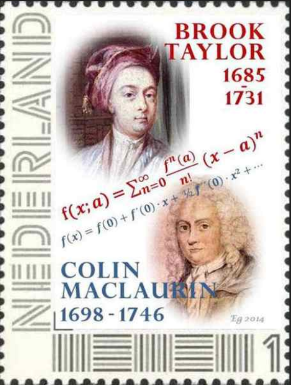
is called the Taylor series for \(f\) expanded about (or centered at) \(a\). Although this systematic “machine” for obtaining power series for a function seems to have been known to a number of mathematicians in the early 1700s, Brook Taylor (1685–1731) was the first to publish this result in his Methodus Incrementorum (1715). The special case when \(a=0\) was included by Colin Maclaurin (1698–1746) in his Treatise of Fluxions (1742). Thus when \(a=0\text{,}\) the series \(\sum_{n=0}^\infty\frac{f^{(n)}(0)}{n!}x^n\) is often called the Maclaurin Series for \(f\text{.}\)
The prime notation for the derivative was not used by Taylor, Maclaurin or their contemporaries. It was introduced by Joseph Louis Lagrange in his 1779 work Thèorie des Fonctions Analytiques. In that work, Lagrange sought to get rid of Leibniz’ infinitesimals and base Calculus on the power series idea. His idea was that by representing every function as a power series, Calculus could be done algebraically by manipulating power series and examining various aspects of the series representation instead of appealing to the controversial notion of infinitesimals. He implicitly assumed that every continuous function could be replaced with its power series representation.
That is, he wanted to think of the Taylor series as a “great big polynomial,” because polynomials are easy to work with. It was a very simple, yet exceedingly clever and far-reaching idea. Since \(e^x = 1 +x +x^2/2 +\ldots\text{,}\) for example, why not just define the exponential to be the series and work with the series. After all, the series is just a very long polynomial.
This idea did not come out of nowhere. Particular infinite series, such as the Geometric Series had been known and studied for many years. Later, in the 18th century Leonhard Euler used infinite series to solve many problems, and some of his solutions are still quite breath–taking when you first see them [16].
Lagrange observed that the coefficient of \((x-a)^n\) provides the \(n\)th derivative of \(f\) at \(a\) (divided by \(n!\)). Modifying formula (4.1.2) to suit his purpose, Lagrange supposed that every differentiable function could be represented as
Apply Lagrange’s idea to determine the \(n\)th derivative of \(\sin x\text{.}\) Compare with the results you get from differentiating \(\sin x\) directly.
In Problem 3.3.3 you determined the power series expansion of \(e^x\) about \(a\text{.}\) Apply Lagrange’s idea to show that every derivative of \(e^x\) is given by \(e^x\text{.}\)
In part (b) of Problem 3.3.1 you determined the power series expansion of \(\ln(x)\) about \(a>0\text{.}\) Apply Lagrange’s idea to show that the derivative of \(\ln (x)\) is \(\frac{1}{x}\text{.}\)
As we observed in Section 3.1 Leibniz and his peers would have regarded the expression \(\dfdx{z}{x}\) as a fraction (of differentials) so they would have derived the formula
by simply canceling the \(\dx{y}\) that appears in the numerator and denominator, just as we did in Section 3.1 (or sometimes by “uncancelling” them to get the left side of equation (4.1.3) from the right side). Mathematicians of that era would have regarded this operation as basic algebra.
Eighteenth and nineteenth century arithmetic primers used the phrase “chain rule” to describe the daisy–chain of symbolic cancellations that occurs when we convert units. For example, to convert yards to inches we compute
Since the cancellations in equation (4.1.3) appeared to be just another example of the older “chain rule” the name was adopted by 20th century Calculus textbooks even though in modern times it is better understood as a mnemonic for the deeper and more abstract operation of computing the derivative of composed functions like \(f(g(x))\text{.}\)
In his Théorie des fonctions analytiques (1797) Lagrange provided a derivation of the Chain Rule in these more modern terms. The following problem captures his idea.
All in all, Lagrange’s idea was very clever and insightful. It’s only real flaw is that the fundamental, underlying assumption is not true. It turns out that not every differentiable function can be represented as a Taylor series. This was demonstrated very dramatically by Augustin Cauchy’s famous counter-example
This function is actually infinitely differentiable everywhere but its Maclaurin series (that is, its Taylor series with \(a=0\)) does not converge to \(f\) (except, trivially, at the origin) because all of its derivatives at the origin are equal to zero. That is \(f^{(n)}(0) = 0, \forall\, n \in
\NN\text{.}\)
Conceptually, it is not difficult to compute these derivatives using the tools you learned in Calculus but the formulas involved do become complicated rather quickly. Some care must be taken to avoid error. To streamline things a bit we take \(y= x^{-1}\text{,}\) and define \(p_2(x) = 4x^6-6x^4\) so that
Unfortunately everything we’ve done so far only gives us the derivatives we need when \(x\) is not zero, and we need the derivatives when \(x\)is zero. To find these we need to get back to very basic ideas.
This example showed that while it was fruitful to exploit Taylor series representations of various functions, basing the foundations of Calculus on power series was not a sound idea.
While Lagrange’s approach wasn’t totally successful, it was a major step away from infinitesimals and toward the modern approach. We still use aspects of it today. For instance we still use his prime notation to denote the derivative.
Turning Lagrange’s idea on its head it is clear that if we know how to compute derivatives, we can use this “machine” to obtain a power series when we are not clever enough to obtain the series by other (typically shorter) means. For example, consider Newton’s binomial series when \(\alpha=\frac{1}{2}\text{.}\) Originally, we obtained this series by extending the binomial theorem to non-integer exponents. Taylor’s formula provides a more systematic procedure. First we compute the derivatives of \(f\) at zero:
As you can see, Taylor’s “machine” will produce the power series for a function (if it has one), but is tedious to perform. We will find, generally, that this tediousness can be an obstacle to understanding. In many cases it will be better, or at least quicker, to be clever if we can. However, it is comforting to have Taylor’s formula available as a last resort.
resembles the Taylor series and, in fact, is called the \(\boldsymbol n\)th degree Taylor polynomial of \(f\) about \(\boldsymbol a\). Theorem 4.1.12 says that a function can be written as the sum of this polynomial and a specific integral which we will analyze in Chapter 7.
We will get the proof started and leave the formal induction proof as an exercise. To begin the induction notice that when \(n=0\)equation (4.1.5) is a restatement of the Fundamental Theorem of Calculus:
Until we began this chapter our approach to series mirrored that of the eighteenth century mathematicians. By exploiting the ideas of Calculus and power series they ingeniously derived mathematical results which were virtually unobtainable before. Mathematicans were eager to push these techniques as far as they could to obtain their results and they often showed good intuition regarding what was mathematically acceptable and what was not. However, as the envelope was pushed further and further, substantial questions about the validity of their methods surfaced.
If we group the terms as follows \((1-1)+(1-1)+\cdots\text{,}\) the series would equal \(0\text{.}\) A regrouping of \(1+(-1+1)+(-1+1)+\cdots\) provides an answer of \(1\text{.}\) This violation of the associative law of addition did not escape the mathematicians of the 1700s. In his 1760 paper On Divergent Series Euler said:
Notable enough, however are the controversies over the series \(1-1+1-1+\text{etc}\text{,}\) whose sum was given by Leibniz as \(\frac{1}{2}\text{,}\) although others disagree . . . Understanding of this question is to be sought in the word “sum;” this idea, if thus conceived — namely, the sum of a series is said to be that quantity to which it is brought closer as more terms of a series are taken — has relevance only for the convergent series, and we should in general give up this idea of sum for divergent series. On the other hand, as series in analysis arise from the expansion of fractions or irrational quantities or even of transcendentals, it will, in turn, be permissible in calculation to substitute in place of such series that quantity out of whose development it is produced.
Even with this formal approach to series, an interesting question arises. The series for the antiderivative of \(\frac{1}{1+x}\) does converge for \(x=1\) while this one does not. Specifically, one antiderivative of the above series is
If we substitute \(x=1\) into this series, we obtain \(\ln
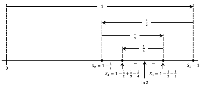
2=1-\frac{1}{2}+\frac{1}{3}-\cdots\text{.}\) It is not hard to see that such an alternating series converges. The following picture shows why. In this diagram, \(S_n\) denotes the partial sum \(1-\frac{1}{2}+\frac{1}{3}-\cdots+\frac{(-1)^{n+1}}{n}\text{.}\)
From the diagram we can see \(S_2\leq S_4\leq S_6\leq\cdots\leq\cdots\leq S_5\leq S_3\leq S_1\) and \(S_{2k+1}-S_{2k}=\frac{1}{2k+1}\text{.}\) It seems that the sequence of partial sums will converge to whatever is in the “middle.” Our diagram indicates that it is ln \(2\) in the middle but actually this is not obvious. Nonetheless it is interesting that one series converges for \(x=1\) but the other does not.
to determine how many terms of the series \(\sum_{n=1}^\infty\frac{(-1)^{n+1}}{n}\) should be added together to approximate \(\ln 2\) to within \(.0001\) without actually computing what \(\ln 2\) is.
These examples illustrate something even more perplexing. As we’ve observed the divergent infinite sum \(1-1+1-1+\cdots\) does not appear satisfy the associative law for addition. Since the sum diverges (is meaningless) this is not too surprising. On the other hand while the convergent series \(1-\frac{1}{2}+\frac{1}{3}-\cdots\) does satisfy the associative law as expected, it does not satisfy the commutative law. In fact, Theorem 4.2.3 shows that it fails, rather spectacularly, to be commutative.
Let \(a\) be any real number. There exists a rearrangement of the Alternating Harmonic Series \(1-\frac{1}{2}+\frac{1}{3}-\cdots\) which converges to \(a\text{.}\)
This says that if we add enough terms of \(-\frac{1}{2}-\frac{1}{4}-\frac{1}{6}-\cdots\) we can make such a sum as large as we wish (and negative) and if we add enough terms of \(1+\frac{1}{3}+\frac{1}{5}+\cdots\) we can make such a sum as large as we wish (and positive). Those facts provide us with the general outline of the proof. The trick is to add just enough positive terms until the sum is just greater than \(a\text{.}\) Then we start to add on negative terms until the sum is just less than \(a\text{.}\) Picking up where we left off with the positive terms, we add on just enough positive terms until we are just above \(a\) again. We then add on negative terms until we are below \(a\text{.}\) In essence, we are bouncing back and forth around \(a\text{.}\) If we do this carefully, then we can get this rearrangement to converge to \(a\text{.}\) The notation in the proof below gets a bit hairy, but keep this general idea in mind as you read through it.
Let \(O_1\) be the first odd integer such that \(1+\frac{1}{3}+\frac{1}{5}+\cdots+\frac{1}{O_1}>a\text{.}\) Now choose \(E_1\) to be the first even integer such that
Continue defining \(O_k\) and \(E_k\) in this fashion for \(k\ge 4\text{.}\) Since \(\limit{k}{\infty}{\frac{1}{O_k}}=\limit{k}{\infty}{\frac{1}{E_k}}=0\text{,}\) it is evident that the partial sums
The two parts of the next problem are extentions of Theorem 4.2.3 but they are a bit simpler notationally since we don’t need to worry about converging to an actual number. We only need to make the rearrangement increase or decrease without bound.
It is fun to know that we can rearrange some series to make them add up to anything we like but there is a more fundamental idea at play here. That the negative terms of the Alternating Harmonic Series diverge to negative infinity and the positive terms diverge to positive infinity make the convergence of the alternating series very special.
Consider what happens when we sum the series. We start with \(1\text{.}\) This is a positive term so our sum is starting to increase without bound. Next we add \(-1/2\) which is a negative terms so our sum has turned around and is now starting to decrease without bound. Then another positive term is added: increasing without bound. Then another negative term: decreasing. And so on. The convergence of the alternating Harmonic Series is the result of a delicate balance between a tendency to run off to positive infinity and back to negative infinity. When viewed in this light it is not really too surprising that rearranging the terms can destroy this delicate balance.
Naturally, the alternating Harmonic Series is not the only such series. Any such series is said to converge conditionally — the condition being the specific arrangement of the terms.
To stir the pot a bit more, some series do satisfy the commutative property. More specifically, one can show that any rearrangement of the series \(1-\frac{1}{2^2}+\frac{1}{3^2}-\cdots\) must converge to the same value as the original series (which happens to be \(\int_{x=0}^1\frac{\ln(1+x)}{x}\dx{x}\approx.8224670334\)). Why does one series behave so nicely whereas the other does not? The answer to that question will have to wait until Section 11.2.
Anomalies like these were well known in the \(1700\)s, but they were overshadowed by the overwhelming utility of the Calculus. Indeed, foundational questions raised by the above examples as well as concerns about the validity of using the infinitely small and infinitely large, while certainly interesting and of importance, did not significantly deter the exploitation of Calculus in studying physical phenomena. However, the envelope eventually was pushed to the point that not even the most practically oriented mathematician could avoid these foundational issues.