Section 9.1 The Nested Interval Property: Completeness of the Real Number System
In deriving the
Lagrange and
Cauchy forms of the remainder for Taylor series, we made use of the
Extreme Value Theorem (
EVT) and
Intermediate Value Theorem (
IVT). In
Chapter 8, we produced an analytic definition of continuity that we can use to prove these theorems. Before we can work out the rest of the tools needed for those proofs we need to explore the make–up of the real number system.
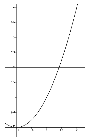
To illustrate what we mean, suppose that we have only the rational number system available. We can still use our definition of continuity and can still consider continuous functions such as
\(f(x)=x^2\text{.}\)
Notice that
\(2\) is a value that lies between
\(f(1)=1\) and
\(f(2)=4\) so the
IVT says that somewhere between
\(1\) and
\(2\text{,}\) \(f\) must take on the value
\(2\text{.}\) That is, there must exist some number
\(c\in[1,2]\) such that
\(f(c)=2\text{.}\) You might say, “Big deal! Everyone knows
\(c=\sqrt{2}\) works.”
However, we are only working with rational numbers and
\(\sqrt{2}\) \(\)is not rational. As we saw in
Chapter 2 the rational number system has holes in it, whereas the real number system doesn’t. Again, “Big deal! Let’s just say that the real number system contains (square) roots.”
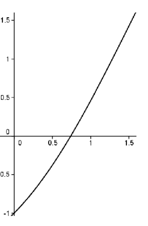
This sounds reasonable and it actually works for square roots, but consider the function
\(f(x)=x-\cos x\text{.}\) We know this is a continuous function (Why?). We also know that
\(f(0)=-1\) and
\(f(\frac{\pi}{2})=\frac{\pi}{2}\text{.}\) Thus according to the
IVT, there should be some number
\(c\in[0,\frac{\pi}{2}]\text{,}\) where
\(f(c)=0\text{.}\) The graph of
\(f(x)=x-\cos x\) is shown below.
The situation is not as transparent as before. What is this mysterious
\(c\) where the curve crosses the
\(x\) axis? Somehow we need to convey the idea that the real number system is a continuum, that it is
complete. That is, it has no holes in it.
How about this? Why don’t we just assume that it has no holes in it? Sometimes the simplest answer works best! We could do that. More complicated statements have been taken as axioms in the past. But how are we going to formulate a rigorous proof based on the statement, “There are no holes in the real numbers”?
Also, going back to the Greeks (and possibly further) the thrust of mathematics has always been to keep our axioms as simple and self–evident as possible and to prove more complicated statements from the axioms. If possible. So we’d prefer to make a simpler assumption (axiom) and use it to show that there are no holes in the real numbers.
We will see that there are several different, but equivalent assumptions we can make that will convey the notion of
completeness. We will explore some of them in this chapter. For now we adopt the following as our
Completeness Axiom for the real number system.
Axiom 9.1.1. Nested Interval Property of the Real Number System (NIP).
Suppose we have two sequences of real numbers
\(\left(x_n\right)\) and
\(\left(y_n\right)\) satisfying the following conditions:
-
\(x_1\leq x_2\leq x_3\leq\ldots\) (this says that the sequence,
\(\left(x_n\right)\text{,}\) is non-decreasing)
-
\(y_1\geq y_2\geq y_3\geq\ldots\) (this says that the sequence,
\(\left(y_n\right)\text{,}\) is non-increasing)
-
\(\forall\ n\text{,}\) \(x_n\leq y_n\)
-
\(\displaystyle \limit{n}{\infty}{\left(y_n-x_n\right)}=0\)
Then there exists a unique number
\(c\) such that
\(x_n\leq c\leq y_n\) for all
\(n\text{.}\)
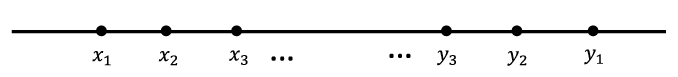
Geometrically, we have the following situation.
Notice that we have two sequences
\(\left(x_n\right)\) and
\(\left(y_n\right)\text{,}\) one increasing (really non-decreasing) and one decreasing (non-increasing). These sequences do not pass each other. In fact, the following is true:
Problem 9.1.2.
Let
\((x_n), (y_n)\) be sequences as in the
NIP. Show that for all
\(n, m \in\NN\text{,}\) \(x_n\le y_m\text{.}\)
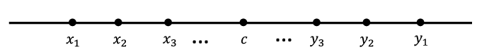
They are also coming together in the sense that
\(\limit{n}{\infty}{\left(y_n-x_n\right)}=0\text{.}\) The
NIP says that in this case there is a unique real number
\(c\) in the middle of all of this:
\(x_n\leq c\leq y_n\) for all
\(n\in\NN\text{.}\)
If there was no such
\(c\) then there would be a hole where these two sequences come together. The
NIP guarantees that there is no such hole. We do not need to prove this since an axiom is, by definition, a self evident truth. We are taking it on faith that the real number system has this property. The next problem shows that the completeness property distinguishes the real number system from the rational number system.
Problem 9.1.3.
(a)
Find two sequences of rational numbers
\(\left(x_n\right)\)and
\(\left(y_n\right)\) which satisfy all four conditions of the
NIP and such that there is no rational number
\(c\) satisfying the conclusion of the
NIP.
Hint.
Consider the decimal expansion of an irrational number.
(b)
Find two sequences of rational numbers
\(\left(x_n\right)\) and
\(\left(y_n\right)\) which satisfy all four conditions of the
NIP and such that there is a rational number
\(c\) satisfying the conclusion of the
NIP.
You might find the name
Nested Interval Property to be somewhat curious since it doesn’t explicitly identify any intervals as such. But in light of
Problem 9.1.2 it should be clear that the sequences
\((x_n)\) and
\((y_n)\) are the left and right endpoints of a set of nested intervals
\([x_1,y_1]\supseteq[x_2,y_2]\supseteq[x_3,y_3]\supseteq\cdots\text{,}\) whose lengths
\(y_n-x_n\) are shrinking to
\(0\text{.}\) The conclusion says that the intersection of these intervals is non–empty and in fact, consists of a single point. That is, it says
\begin{equation*}
\bigcap_{n=1}^\infty[x_n,y_n]=\{c\}\text{.}
\end{equation*}
Intuitively, the sequences
\(\left(x_n\right)\) and
\(\left(y_n\right)\) in the
NIP appear to converge to
\(c\text{.}\) This is in fact, true and can be proven rigorously. This will prove to be a valuable piece of information for us.
Theorem 9.1.4.
Suppose that we have two sequences \(\left(x_n\right)\) and \(\left(y_n\right)\) satisfying all of the assumptions of the Nested Interval Property. If \(c\) is the unique number such that \(x_n\leq c\leq y_n\) for all \(n\text{,}\) then
\begin{equation*}
\limit{n}{\infty}{x_n}=c = \limit{n}{\infty}{y_n}\text{.}
\end{equation*}
Problem 9.1.5.
To illustrate the idea that the
NIP plugs the holes in the real line, we will prove the existence of square roots of non–negative real numbers.
Theorem 9.1.6.
Suppose
\(a\in\mathbb{R},\,a\geq 0\text{.}\) There exists a real number
\(c\geq 0\) such that
\(c^2=a\text{.}\)
Notice that we can’t just say, “Let
\(c=\sqrt{a}\text{,}\)” since the idea is to show that this square root exists. In fact, throughout this proof, we cannot really use a square root symbol as we haven’t yet proved that square roots exist. The idea behind the proof illustrates how the
NIP is used in practice.
Sketch of Proof.
Our strategy is to construct two sequences which will narrow in on the number
\(c\) that we seek. Observe that we need to find a number
\(x_1\) such that
\(x_1^2\leq a\) and a number
\(y_1\) such that
\(y_1^2\geq a\text{.}\) (Remember that we can’t say
\(x_1\lt\sqrt{a}\) and
\(y_1\gt\sqrt{a}\) since our goal is to show that
\(\sqrt{a} \) exists.) There are many possibilities, but how about
\(x_1=0\) and
\(y_1=a+1?\) You can check that these will satisfy
\(x_1^2\leq a\leq\) \(y_1^2\text{.}\) Furthermore
\(x_1\leq
y_1\text{.}\) This is the starting point.
The technique we will employ is often called a bisection technique, and is a useful way to set ourselves up for applying the
NIP. Let
\(m_1\) be the midpoint of the interval
\([\,x_1,y_1]\text{.}\) Then either we have
\(m_1^2\leq
a\) or
\(m_1^2\geq a\text{.}\) In the case
\(m_1^2\leq a\text{,}\) we really want
\(m_1\) to take the place of
\(x_1\) since it is larger than
\(\,x_1\text{,}\) but still represents an underestimate for what would be the square root of
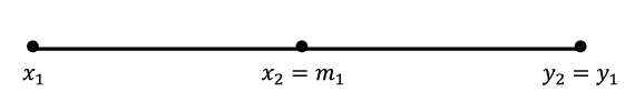
\(a\text{.}\) This thinking prompts the following move. If
\(m_1^2\leq
a\text{,}\) we will relabel things by letting
\(x_2=m_1\) and
\(y_2=y_1\text{.}\) The situation looks like this on the number line.
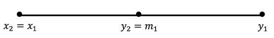
In the other case where
\(a\leq m_1^2\text{,}\) we will relabel things by letting
\(x_2=x_1\) and
\(y_2=m_1\text{.}\) The situation looks like this on the number line.
In either case, we’ve reduced the length of the interval where the square root lies to half the size it was before. Stated in more specific terms, in either case we have the same results:
\begin{align*}
x_1\leq x_2\leq y_2\leq y_1,
\amp{} \amp{}
x_1^2\leq a\leq y_1^2,
\amp{}\amp{}
x_2^2\leq a\leq y_2^2,
\end{align*}
and
\begin{align*}
\amp{}
y_2-x_2=\frac{1}{2}\left(y_1-x_1\right).
\end{align*}
Now we play the same game, but instead we start with the interval \([x_2,y_2]\text{.}\) Let \(m_2\) be the midpoint of \([x_2,y_2]\text{.}\) Then we have \(m_2^2\leq a\) or \(m_2^2\geq a\text{.}\) If \(m_2^2\leq a\text{,}\) we relabel \(x_3=m_2\) and \(y_3=y_2\text{.}\) If \(a\leq m_2^2\text{,}\) we relabel \(x_3=x_2\) and \(y_3=m_2\text{.}\) In either case, we end up with
\begin{equation*}
x_1\leq x_2\leq x_3\leq y_3\leq y_2\leq y_1,
\end{equation*}
\begin{align*}
x_1^2\leq a\leq y_1^2,
\amp{}\amp{}
x_2^2\leq a\leq y_2^2,
\amp{}\amp{}
x_3^2\leq a\leq y_3^2,
\end{align*}
and
\begin{gather*}
y_3-x_3=\frac{1}{2}\left(y_2-x_2\right)=\frac{1}{2^2}\left(y_1-x_1\right).
\end{gather*}
Continuing in this manner, will produce two sequences, \(\left(x_n\right)\)and \(\left(y_n\right)\) satisfying the following conditions:
- Condition 1:
-
\(\displaystyle x_1\leq x_2\leq x_3\leq\ldots\)
- Condition 2:
-
\(\displaystyle y_1\geq y_2\geq y_3\geq\ldots\)
- Condition 3:
-
\(\forall\ n\text{,}\) \(x_n\leq y_n\)
- Condition 4:
-
\(\displaystyle \limit{n}{\infty}{\left(y_n-x_n\right)}=\limit{n}{\infty}{\left[\frac{1}{2^{n-1}}\left(y_1-x_1\right)\right]}=0\)
- Condition 5:
-
These sequences also satisfy the following property:
\begin{equation*}
\forall\ n, x_n^2\leq a\leq y_n^2
\end{equation*}
Conditions 1 through 4 tell us that
\(\left(x_n\right)\)and
\(\left(y_n\right)\) satisfy all of the conditions of the
NIP, so we can conclude that there must exist a real number
\(c\) such that
\(x_n\leq c\leq y_n\) for all
\(n\text{.}\) At this point, you should be able to use Condition 5. to show that
\(c^2=a\) as desired.
Problem 9.1.7.
The bisection method we employed to prove
Theorem 9.1.6 is also pretty typical of how we will use the
NIP, as it ensures that we will create a sequence of nested intervals which meet all of the conditions specified in the
NIP. We will employ this strategy in the proofs of the
IVT and
EVT. Deciding how to relabel the endpoints of our intervals will be determined by what we want to do with these two sequences of real numbers. This will typically lead to a fifth property, which will be crucial in proving that the
\(c\) guaranteed by the
NIP does what we want it to do. Specifically, in the above example, we always wanted our candidate for
\(\sqrt{a}\) to be in the interval
\([\,x_n,y_n]\text{.}\) This judicious choice led to the extra Condition 5:
\(\forall\) \(n,\,x_n^2\leq a\leq y_n^2\text{.}\) In applying the
NIP to prove the
IVT and
EVT, Condition 5 is what will change based on the property we want
\(c\) to have.
Before we tackle the
IVT and
EVT, let’s use the
NIP to address an interesting question about the Harmonic Series. Recall that the Harmonic Series,
\(1+\frac{1}{2}+\frac{1}{3}+\frac{1}{4}+\cdots\text{,}\) grows without bound. That is,
\(\sum_{n=1}^\infty\frac{1}{n}=\infty\text{.}\) The question is how slowly does this series grow? For example, how many terms would it take before the series surpasses 100? Or 1000? Or 10000?
Leonhard Euler decided to tackle this problem in the following way. He decided to consider the
\begin{equation}
\limit{n}{\infty}{\left[\left(1+\frac{1}{2}+\frac{1}{3}+\cdots+
\frac{1}{n}\right)-\ln(n+1)\right]} \text{.}\tag{9.1.1}
\end{equation}
This limit is called Euler’s constant and is traditionally denoted by
\(\gamma\text{.}\) Equation (9.1.1) says that for very large values of
\(n\text{,}\) we have
\begin{equation*}
1+\frac{1}{2}+\frac{1}{3}+\cdots+\frac{1}{n}\approx
\ln\left(n+1\right)+\gamma\text{.}
\end{equation*}
If we could approximate \(\gamma\text{,}\) then we could replace the inequality \(1+\frac{1}{2}+\frac{1}{3}+\cdots+\frac{1}{n}\geq 100\) with the more tractable inequality ln\(\left(n+1\right)+\gamma\) \(\geq 0\) and solve for \(n\) in this. This should tell us roughly how many terms would need to be added in the Harmonic Series to surpass 100. Approximating \(\gamma\) with a computer is not too bad. We could make \(n\) as large as we wish in \(\left(1+\frac{1}{2}+\frac{1}{3}+\cdots+\frac{1}{n}\right)-\)ln\(\left(1+n\right)\) to make closer approximations for \(\gamma\text{.}\) The real issue is, how do we know that
\begin{equation*}
\limit{n}{\infty}{\left[\left(1+\frac{1}{2}+\frac{1}{3}+\cdots+
\frac{1}{n}\right)-\ln(n+1)\right]}
\end{equation*}
actually exists? As of the time we are writing this book it is not even known if \(\gamma\) is rational or irrational. So in our opinion, the existence of this limit is not obvious. And even if it were, a formal proof would be required.
We will use the
NIP to show that this limit does in fact exist. The details are in the following problem.
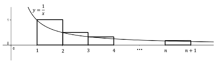
Problem 9.1.8.
(a)
Let \(x_n=\left(1+\frac{1}{2}+\frac{1}{3}+\cdots+\frac{1}{n}\right)-\ln\left(n+1
\right)\text{.}\) Use the following diagram to show
\begin{equation*}
x_1\leq x_2\leq x_3\leq\cdots
\end{equation*}
(b)
Let
\(z_n=\ln\left(n+1\right)-\left(\frac{1}{2}+\frac{1}{3}+\cdots+\frac{1}{n+1}
\right)\text{.}\) Use a similar diagram to show that
\(z_1\leq z_2\leq z_3\leq\cdots\text{.}\)
(c)
Let
\(y_n=1-z_n\text{.}\) Show that
\(\left(x_n\right)\) and
\(\left(y_n\right)\) satisfy the hypotheses of the nested interval property and use the
NIP to conclude that there is a real number
\(\gamma\) such that
\(x_n\leq\gamma\leq y_n\) for all
\(n\text{.}\)
(d)
Conclude that
\(\limit{n}{\infty}{\left[\left(1+\frac{1}{2}+\frac{1}{3}+\cdots+
\frac{1}{n}\right)-\ln\left(n+1\right)\right]}=\gamma\text{.}\)
Problem 9.1.9.
(a)
Use the inequality
\(x_n\leq\gamma\leq y_n\) for all
\(n\) to approximate
\(\gamma\) to three decimal places.
(b)
Use the fact that for large \(n\text{,}\) \(1+\frac{1}{2}+\frac{1}{3}+\cdots+\frac{1}{n}\approx
\ln\left(n+1\right)+ \gamma\) to determine approximately how large \(n\) must be to make
\begin{equation*}
1+\frac{1}{2}+\frac{1}{3}+\cdots+\frac{1}{n}\geq 100\text{.}
\end{equation*}
(c)
Suppose we have a supercomputer which can add
\(10\) trillion terms of the Harmonic Series per second. Approximately how many times the current age of the Earth would it take for this computer to sum the Harmonic Series until it surpasses
\(100\text{?}\)
Section 9.3 The Bolzano–Weierstrass Theorem
Theorem 9.3.1.
A continuous function defined on a closed, bounded interval must be bounded. That is, let
\(f\) be a continuous function defined on
\([\,a,b]\text{.}\) Then there exists a positive real number
\(B\) such that
\(|f(x)|\leq B\) for all
\(x\in[\,a,b]\text{.}\)
Sketch of Alleged Proof: Let’s assume, for contradiction, that there is no such bound
\(B\text{.}\) This says that for any positive integer
\(n\text{,}\) there must exist
\(x_n\in[a,b]\) such that
\(\abs{f(x_n)}>n\text{.}\) (Otherwise
\(n\) would be a bound for
\(f\text{.}\))
IF the sequence
\(\left(x_n\right)\) converges to, say
\(c\in[a,b]\text{,}\) then we would have our contradiction. Indeed, we would have
\(\limit{n}{\infty}{x_n}=c\text{,}\) and by the continuity of
\(f\) at
\(c\) and
Theorem 8.2.1 we would have
\(\limit{n}{\infty}{f(x_n)}=f(c)\) which implies that the sequence
\(\left(f(x_n)\right)\) converges. So by
Lemma 6.2.7 the sequence
\(\left(f(x_n)\right)\) must be bounded. This would provide our contradiction since, by construction
\(\abs{f(x_n)}\gt{}n\text{,}\) for all positive integers
\(n\text{.}\) QED?
This would work well except for one little problem. The way it was constructed, there is no reason to expect the sequence
\(\left(x_n\right)\) to converge to anything That is why we emphasized the
IF above. Fortunately, this idea can be salvaged. While it is true that the sequence
\(\left(x_n\right)\) may not converge, part of it will. We will need the following definition.
Definition 9.3.2.
Let
\(\left(n_k\right)_{k=1}^\infty\) be a strictly increasing sequence of positive integers; that is,
\(n_1\lt n_2\lt n_3\lt \cdots\) . If
\(\left(x_n\right)_{n=1}^\infty\) is a sequence, then
\(\left(x_{n_k}\right)_{k=1}^\infty=\left(x_{n_1},x_{n_2},x_{n_3},\ldots \right)\) is called a subsequence of
\(\left(x_n\right)\text{.}\)
The idea is that a subsequence of a sequence is a part of the sequence,
\((x_n)\text{,}\) which is itself a sequence. However, it is a little more restrictive. We can choose any term in our sequence to be part of the subsequence, but once we choose that term, we can’t go backwards. This is where the condition
\(n_1\lt n_2\lt n_3\lt \cdots\) comes in. For example, suppose we started our subsequence with the term
\(x_{100}\text{.}\) We could not choose our next term to be
\(x_{99}\text{.}\) The subscript of the next term would have to be greater than 100. In fact, the thing about a subsequence is that it is all in the subscripts; we are really choosing a subsequence
\(\left(n_k\right)\) of the sequence of subscripts
\(\left(n\right)\) in
\(\left(x_n\right)\text{.}\)
Example 9.3.3.
Given the sequence
\(\left(x_n\right)\text{,}\) the following are subsequences.
(a)
\(\left(x_2,\,x_4,\,x_6,\,\ldots\right)=\left(x_{2k}\right)_{k=1}^\infty\)
(b)
\(\left(x_1,\,x_4,\,x_9,\,\ldots\right)=\left(x_{k^2}\right)_{k=1}^ \infty\)
(c)
\(\left(x_n\right)\) itself.
Example 9.3.4.
The following are
NOT subsequences.
(a)
\(\left(x_1,\,x_1,\,x_1,\,\ldots\right)\)
(b)
\(\left(x_{99},\,x_{100},\,x_{99},\,\ldots\right)\)
(c)
\(\left(x_1,\,x_2,\,x_3\right)\)
The subscripts in the examples we have seen so far have a discernable pattern, but this need not be the case. For example,
\begin{equation*}
\left(x_2,\,x_5,\,x_{12},\,x_{14},\,x_{23},\,\ldots\right)
\end{equation*}
would be a subsequence as long as the subscripts form an increasing sequence themselves.
Problem 9.3.5.
Suppose
\(\limit{n}{\infty}{x_n}=c\text{.}\) Prove that
\(\limit{k}{\infty}{x_{n_k}}=c\) for any subsequence
\(\left(x_{n_k}\right)\) of
\(\left(x_n\right)\text{.}\)
Hint.
First prove that
\(n_k\geq k\text{.}\)
A very important theorem about subsequences was introduced by Bernhard Bolzano and was later proven independently by Karl Weierstrass. Basically, this theorem says that any bounded sequence of real numbers has a convergent subsequence.
Theorem 9.3.6. The Bolzano–Weierstrass Theorem.
Let
\(\left(x_n\right)\) be a sequence of real numbers such that
\(x_n\in[\,a,b]\text{,}\) \(\forall\) \(n\text{.}\) Then there exists
\(c\in[\,a,b]\) and a subsequence
\(\left(x_{n_k}\right)\text{,}\) such that
\(\limit{k}{\infty}{x_{n_k}}=c\text{.}\)
As an example of this theorem, consider the sequence
\begin{equation*}
\left((-1)^n\right)=\left(-1,1,-1,1,\ldots\right) \text{.}
\end{equation*}
This sequence does not converge, but the subsequence
\begin{equation*}
\left((-1)^{2k}\right)=\left(1,1,1,\ldots\right)
\end{equation*}
converges to \(1\text{.}\) This is not the only convergent subsequence. For example, the subsequence
\begin{equation*}
\left((-1)^{2k+1}\right)=(-1,-1,-1,\,\ldots)
\end{equation*}
also converges to \(-1\text{.}\) Notice that if the sequence is unbounded, then all bets are off. The sequence may have a convergent subsequence or it may not. The sequences
\begin{align*}
\left(\left((-1)^n+1\right)n\right) \amp{}\amp{}\text{ and }
\amp{}\amp{}\left(n\right)
\end{align*}
represent these possibilities as the first contains for example, the convergent subsequence \(\left(\left((-1)^{2k+1}+1\right)(2k+1)\right)=(0,0,0,\ldots)\) and all subsequences of the the second diverge to infinity.
The Bolzano–Weierstrass Theorem says that no matter how the sequence
\(\left(x_n\right)\) is produced, as long as it is bounded then it contains a convergent subsequence. This can be very useful. In particular the sequence
\((x_n)\) that appears in our Alleged Proof is bounded since
\(x_n\in [a,b]\
\forall \ n\in\NN\text{.}\) So it contains a convergent subsequence.
Sketch of a Proof of the Bolzano–Weierstrass Theorem.
Suppose we have our sequence
\(\left(x_n\right)\) such that
\(x_n\in[a,b]\text{,}\) \(\forall\) \(n\text{,}\) as in the Alleged Proof above. We will use the
NIP to find a convergent subsequence
\(\left( x_{n_k}\right) \) and the value
\(c\) that it will converge to. Since we are already using
\(\left(x_n\right)\) as our original sequence, we will need to use different letters in setting ourselves up for the
NIP. With this in mind, let
\(a_1=a\) and
\(b_1=b\text{,}\) and notice that
\(x_n\in[a_1,b_1]\) for infinitely many
\(n\text{.}\) (This is, in fact true for all
\(n\text{,}\) but you’ll see why we said it the way we did.) Let
\(m_1\) be the midpoint of
\([a_1,b_1]\) and notice that either
\(x_n\in[a_1,m_1]\) for infinitely many
\(n\) or
\(x_n\in[m_1,b_1]\) for infinitely many
\(n\text{.}\) If
\(x_n\in[a_1,m_1]\) for infinitely many
\(n\text{,}\) then we relabel
\(a_2=a_1\) and
\(b_2=m_1\text{.}\) If
\(x_n\in[m_1,b_1]\) for infinitely many
\(n\text{,}\) then relabel
\(a_2=m_1\) and
\(b_2=b_1\text{.}\) In either case, we get
\(a_1\leq a_2\leq b_2\leq b_1\text{,}\) \(b_2-a_2=\frac{1}{2}\left(b_1-a_1\right)\text{,}\) and
\(x_n\in[a_2,b_2]\) for infinitely many
\(n\text{.}\)
Now we consider the interval
\([a_2,b_2]\) and let
\(m_2\) be the midpoint of
\([a_2,b_2]\text{.}\) Since
\(x_n\in[a_2,b_2]\) for infinitely many
\(n\text{,}\) then either
\(x_n\in[a_2,m_2]\) for infinitely many
\(n\) or
\(x_n\in[m_2,b_2]\) for infinitely many
\(n\text{.}\) If
\(x_n\in[a_2,m_2]\) for infinitely many
\(n\text{,}\) then we relabel
\(a_3=a_2\) and
\(b_3=m_2\text{.}\) If
\(x_n\in[m_2,b_2]\) for infinitely many
\(n\text{,}\) then we relabel
\(a_3=m_2\) and
\(b_3=b_2\text{.}\) In either case, we get
\(a_1\leq a_2\leq a_3\leq b_3\leq b_2\leq b_1\text{,}\) \(b_3-a_3=\frac{1}{2}\left(b_2-a_2\right)=\frac{1}{2^2}\left(b_1-a_1\right)\text{,}\) and
\(x_n\in[a_3,b_3]\) for infinitely many
\(n\text{.}\)
If we continue in this manner, we will produce two sequences \(\left(a_k\right)\)and \(\left(b_k\right)\) with the following properties:
-
\(\displaystyle a_1\leq a_2\leq a_3\leq\cdots\)
-
\(\displaystyle b_1\geq b_2\geq b_3\geq\cdots\)
-
\(\forall\ k\text{,}\) \(a_k\leq b_k\)
-
\(\displaystyle \displaystyle\limit{k}{\infty}{\left(b_k-a_k\right)}=\limit{k}{\infty}{\left[
\frac{1}{2^{k-1}}\left(b_1-a_1\right)\right]}=0\)
-
For each
\(k\text{,}\) \(x_n\in[\,a_k,b_k]\) for infinitely many
\(n\)
By properties 1-4 and the
NIP, there exists a unique
\(c\) such that
\(c\in[a_k,b_k]\text{,}\) for all
\(k\text{.}\) In particular,
\(c\in[a_1,b_1]=[a,b]\text{.}\)
We have our
\(c\text{.}\) Now we need to construct a subsequence converging to it. Since
\(x_n\in[a_1,b_1]\) for infinitely many
\(n\text{,}\) choose an integer
\(n_1\) such that
\(x_{n_1}\in[a_1,b_1]\text{.}\) Since
\(x_n\in[a_2,b_2]\) for infinitely many
\(n\text{,}\) choose an integer
\(n_2>n_1\) such that
\(x_{n_2}\in[a_2,b_2]\text{.}\) (Notice that to make a subsequence it is crucial that
\(n_2>n_1\text{,}\) and this is why we needed to insist that
\(x_n\in[a_2,b_2]\) for infinitely many
\(n\text{.}\)) Continuing in this manner, we should be able to build a subsequence
\(\left(x_{n_k}\right)\) that will converge to
\(c\text{.}\) You can supply the details in the following problem.
Problem 9.3.7.
Turn the ideas of the above outline into a formal proof of the Bolzano–Weierstrass Theorem.
Problem 9.3.8.
Use the Bolzano–Weierstrass Theorem to complete the proof of
Theorem 9.3.1.
Section 9.4 The Supremum and the Extreme Value Theorem
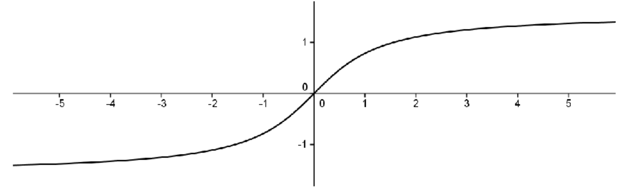
Theorem 9.3.1 says that a continuous function on a closed, bounded interval must be bounded. Boundedness, in and of itself, does not ensure the existence of a maximum or minimum. We must also have a closed, bounded interval. To illustrate this, consider the continuous function
\(f(x)=\)tan
\(^{-1}x\) defined on the (unbounded) interval
\(\left(-\infty,\infty\right)\text{.}\)
This function is bounded between
\(-\frac{\pi}{2}\)and
\(\frac{\pi}{2}\text{,}\) but it does not attain a maximum or minimum as the lines
\(y=\pm\frac{\pi}{2}\) are horizontal asymptotes. Notice that if we restricted the domain to a closed, bounded interval then it would attain its extreme values on that interval (as guaranteed by the
EVT).
To find a maximum we need to find the smallest possible upper bound for the range of the function. This prompts the following definitions.
Definition 9.4.1.
Let
\(S\subseteq\mathbb{R}\) and let
\(b\) be a real number. We say that
\(b\) is an upper bound of
\(S\) provided
\(b\geq x\) for all
\(x\in S\text{.}\)
For example, if
\(S=(0,1)\text{,}\) then any
\(b\) with
\(b\geq 1\) would be an upper bound of
\(S\text{.}\) Furthermore, the fact that
\(b\) is not an element of the set
\(S\) is immaterial. Indeed, if
\(T=[\,0,1]\text{,}\) then any
\(b\) with
\(b\geq 1\) would still be an upper bound of
\(T\text{.}\) Notice that, in general, if a set has an upper bound, then it has infinitely many since any number larger than that upper bound would also be an upper bound. However, there is something special about the smallest upper bound.
Definition 9.4.2. Least Upper Bound.
Let
\(S\subseteq\mathbb{R}\) and let
\(b\) be a real number. We say that
\(b\) is the
least upper bound of
\(S\) provided
-
\(b\geq x\) for all
\(x\in S\text{.}\) (
\(b\) is an upper bound of
\(S\))
-
If
\(c\geq x\) for all
\(x\in S\text{,}\) then
\(c\geq b\text{.}\) (Any upper bound of
\(S\) is at least as big as
\(b\text{.}\))
In this case, we also say that \(b\) is the supremum of \(S\) and we write
\begin{equation*}
b=\sup S\text{.}
\end{equation*}
Notice that the definition really says that \(b\) is the smallest upper bound of \(S\text{.}\) Also notice that the second condition can be replaced by its contrapositive so we can say that \(b=\sup S\) if and only if
-
\(\displaystyle b\,\geq\,x\text{ for all } x\,\in S\)
-
If
\(c\,\lt \,b\) then there exists
\(x\,\in S\) such that
\(c\,\lt \,x\text{.}\)
The second condition says that if a number
\(c\) is less than
\(b\text{,}\) then it can’t be an upper bound, so that
\(b\) really is the smallest upper bound.
Also notice that the supremum of the set may or may not be in the set itself. This is illustrated by the examples above as in both cases,
\(1=\sup(0,1)\) and
\(1=\sup [0,1]\text{.}\) Obviously, a set which is not bounded above such as
\(\mathbb{N}=\{1,\,2,\,3,\,\ldots\}\) cannot have a supremum. However, for non-empty sets which are bounded above, we have the following.
Theorem 9.4.3. The Least Upper Bound Property (LUBP).
Let
\(S\) be a non–empty subset of
\(\mathbb{R}\) which is bounded above. Then
\(S\) has a supremum.
Sketch of Proof.
Since \(S\neq\emptyset\text{,}\) then there exists \(s\in S\text{.}\) Since \(S\) is bounded above then it has an upper bound, say \(b\text{.}\) We will set ourselves up to use the Nested Interval Property. With this in mind, let \(x_1=s\) and \(y_1=b\) and notice that \(\exists\) \(x\in S\) such that \(x\geq x_1\) (namely, \(x_1\) itself) and \(\forall\,x\in S\text{,}\) \(y_1\geq x\text{.}\) You probably guessed what’s coming next: let \(m_1\) be the midpoint of \([\,x_1,y_1]\text{.}\) Notice that either \(m_1\geq x,\,\forall\,x\in S\) or \(\exists\) \(x\in S\) such that \(x\geq m_1\text{.}\) In the former case, we relabel, letting \(x_2=x_1\) and \(y_2=m_1\text{.}\) In the latter case, we let \(x_2=m_1\) and \(y_2=y_1\text{.}\) In either case, we end up with \(x_1\leq x_2\leq y_2\leq y_1\text{,}\) \(y_2-x_2=\frac{1}{2}\left(y_1-x_1\right)\text{,}\) and \(\exists\) \(x\in S\) such that \(x\geq x_2\) and \(\forall\,x\in S\text{,}\) \(y_2\geq x\text{.}\) If we continue this process, we end up with two sequences, \(\left(x_n\right)\)and \(\left(y_n\right)\text{,}\) satisfying the following conditions:
-
\(\displaystyle x_1\leq x_2\leq x_3\leq\ldots\)
-
\(\displaystyle y_1\geq y_2\geq y_3\geq\ldots\)
-
\(\forall\ n\text{,}\) \(x_n\leq y_n\)
-
\(\displaystyle \limit{n}{\infty}{\left(y_n-x_n\right)}=\limit{n}{\infty}{
\left[\frac{1}{2^{n-1}}\left(y_1-x_1\right)\right]}=0\)
-
\(\forall\ n,\exists\ x\in S\) such that
\(x\geq x_n\) and
\(\forall\ x\in S\text{,}\) \(y_n\geq x\text{,}\)
By properties 1–4 and the
NIP there exists
\(c\) such that
\(x_n\leq c\leq y_n,\,\forall\,n\text{.}\) We will leave it to you to use property 5 to show that
\(c=\sup S\text{.}\)
Problem 9.4.4.
Complete the above ideas to provide a formal proof of
Theorem 9.4.3.
Notice that we really used the fact that
\(S\) was non-empty and bounded above in the proof of
Theorem 9.4.3. This makes sense, since a set which is not bounded above cannot possibly have a least upper bound. In fact, any real number is an upper bound of the empty set so that the empty set would not have a least upper bound.
Corollary 9.4.5.
Let
\((x_n)\) be a bounded, increasing sequence of real numbers. That is,
\(x_1\leq x_2\leq x_3\leq\cdots\text{.}\) Then
\((x_n)\) converges to some real number
\(c\text{.}\)
Problem 9.4.6.
Hint.
Let
\(c=\sup\{x_n|\,n=1,2,3,\ldots\}\text{.}\) To show that
\(\limit{n}{\infty}{x_n}=c\text{,}\) let
\(\eps >0.\)Note that
\(c-\eps \) is not an upper bound. You take it from here!
Problem 9.4.7.
Consider the following curious expression
\begin{equation*}
\sqrt{2+\sqrt{2+\sqrt{2+\sqrt{...}}}}\text{.}
\end{equation*}
We will use
Corollary 9.4.5 to show that this actually converges to some real number. After we know it converges we can actually compute what it is. Of course to do so, we need to define things a bit more precisely. With this in mind consider the following sequence
\(\left(x_n\right)\) defined as follows:
\begin{equation*}
x_1=\sqrt{2}
\end{equation*}
\begin{equation*}
x_{n+1}=\sqrt{2+x_n}\text{.}
\end{equation*}
(a)
Use induction to show that
\(x_n\lt 2\) for
\(n=1,\,2,\,3,\,\ldots\text{.}\)
(b)
Use the result from part (a) to show that
\(x_n\lt x_{n+1}\) for
\(n=1,\,2,\,3,\,\ldots\) .
(c)
From
Corollary 9.4.5, we have that
\(\left(x_n\right)\) must converge to some number
\(c\text{.}\) Use the fact that
\(\left(x_{n+1}\right)\) must converge to
\(c\) as well to compute what
\(c\) must be.
Problem 9.4.8.
Let
\(S\subseteq\RR\) and let
\(T=\{-x|\,x\in S\}\text{.}\)
(a)
Mimic the definitions of an upper bound of a set and the least upper bound (supremum) of a set to give definitions for a lower bound of a set and the greatest lower bound (infimum) of a set.
Note: The infimum of a set
\(S\) is denoted by
\(\inf S\text{.}\)
(b)
Prove that
\(b\) is an upper bound of
\(S\) if and only if
\(-b\) is a lower bound of
\(T\text{.}\)
(c)
Prove that
\(b=\sup S\) if and only if
\(-b=\inf T\text{.}\)
(d)
Use parts (b) and (c) to show that the real number system satisfies the
Greatest Lower Bound Property: Any non–empty subset of real numbers which is bounded below has an infimum.
Problem 9.4.9.
Find the least upper bound (supremum) and greatest lower bound (infimum) of the following sets of real numbers, if they exist. (If one does not exist then say so.)
(a)
\(S=\left\{\frac{1}{n}\,|\,n=1,2,3,\ldots\right\}\)
(b)
\(T=\left\{r\,|\,r\right.\) is rational and
\(\left.r^2\lt 2\right\}\)
(c)
\((-\infty,0)\cup(1,\infty)\)
(d)
\(R=\left\{\frac{(-1)^n}{n}\,|\,n=1,2,3,\ldots\right\}\)
(e)
(f)
The empty set
\(\emptyset\)
We now have all the tools we need to tackle the Extreme Value Theorem.
Theorem 9.4.10. Extreme Value Theorem (EVT).
Suppose
\(f\) is continuous on
\([a,b]\text{.}\) Then there exists
\(c,d\in[a,b]\) such that
\(f(d)\leq f(x)\leq f(c)\text{,}\) for all
\(x\in[a,b]\text{.}\)
Sketch of Proof.
We will first show that
\(f\) attains its maximum. To this end, recall that
Theorem 9.3.1 tells us that
\(f[\,a,b]=\{f(x)|\,x\in[\,a,b]\}\) is a non–empty, bounded set. By the
LUBP,
\(f[a,b]\) must have a least upper bound which we will label
\(s\text{,}\) so that
\(s=\sup
f[a,b]\text{.}\) This says that
\(s\geq f(x)\text{,}\)for all
\(x\in[a,b]\text{.}\) All we need to do now is find a
\(c\in[\,a,b]\) with
\(f(c)=s\text{.}\) With this in mind, notice that since
\(s=\sup f[\,a,b]\text{,}\) then for any positive integer
\(n\text{,}\) \(s-\frac{1}{n}\) is not an upper bound of
\(f[\,a,b]\text{.}\) Thus there exists
\(x_n\in[\,a,b]\) with
\(\,s-\frac{1}{n}\lt f(x_n)\leq
s\text{.}\) Now, by the
Bolzano–Weierstrass Theorem,
\(\left(x_n\right)\) has a convergent subsequence
\(\,\left(x_{n_k}\right)\) converging to some
\(c\in[\,a,b]\text{.}\) Using the continuity of
\(f\) at
\(c\text{,}\) you should be able to show that
\(f(c)=s\text{.}\) To find the minimum of
\(f\text{,}\) find the maximum of
\(-f\text{.}\)
Problem 9.4.11.
Formalize the above ideas into a proof of the
EVT.
Notice that we used the
NIP to prove both the
Bolzano–Weierstrass Theorem and the
LUBP. This is really unavoidable, as it turns out that all of those statements are equivalent in the sense that any one of them can be taken as the completeness axiom for the real number system and the others proved as theorems. This is not uncommon in mathematics, as people tend to gravitate toward ideas that suit the particular problem they are working on. In this case, people realized at some point that they needed some sort of completeness property for the real number system to prove various theorems. Each individual’s formulation of completeness fit in with his understanding of the problem at hand. Only in hindsight do we see that they were really talking about the same concept: the completeness of the real number system. In point of fact, most modern textbooks use the
LUBP as the axiom of completeness and prove all other formulations as theorems. We will finish this section by showing that either the
Bolzano–Weierstrass Theorem or the
LUBP can be used to prove the
NIP. This says that they are all equivalent and that any one of them could be taken as the completeness axiom.
Problem 9.4.12.
Use the
Bolzano–Weierstrass Theorem to prove the
NIP. That is, assume that the Bolzano–Weierstrass Theorem holds and suppose we have two sequences of real numbers,
\(\left(x_n\right)\) and
\(\left(y_n\right)\text{,}\) satisfying:
-
\(\displaystyle x_1\le x_2 \le x_3 \le \ldots\)
-
\(\displaystyle y_1\ge y_2 \ge y_3 \ge \ldots\)
-
\(\displaystyle \forall\ n,\ x_n\le y_n\)
-
\(\limit{n}{\infty}{\left(y_n-x_n\right)} = 0\text{.}\)
Prove that there is a unique real number
\(c\) such that
\(x_n\le c\le y_n\text{,}\) for all
\(n\text{.}\)
Problem 9.4.13.
Find a bounded sequence of rational numbers such that no subsequence of it converges to a rational number.
Problem 9.4.14.
Use the
Least Upper Bound Property to prove the
Nested Interval Property. That is, assume that every non-empty subset of the real numbers which is bounded above has a least upper bound; and suppose that we have two sequences of real numbers
\(\left(x_n\right)\) and
\(\left(y_n\right)\text{,}\) satisfying:
-
\(\displaystyle x_1\le x_2 \le x_3 \le \ldots\)
-
\(\displaystyle y_1\ge y_2 \ge y_3 \ge \ldots\)
-
\(\displaystyle \forall\ n, x_n\le y_n\)
-
\(\limit{n}{\infty}{\left(y_n-x_n\right)} = 0\text{.}\)
Prove that there is a unique real number
\(c\) such that
\(x_n\le c\le y_n\text{,}\) for all n.
Problem 9.4.15.
Since the
LUBP is equivalent to the
NIP it does not hold for the rational number system. Demonstrate this by finding a non–empty set of rational numbers which is bounded above, but whose supremum is an irrational number.
We now have the machinery in place to prove the
Archimedean Property of the real number system as we promised we’d to back in
Chapter 2. We mentioned in
Chapter 2, that until the invention of Calculus this was taken to be intuitively obvious but we can now prove it as a formal theorem. The proof depends on the completeness of the real number system.
Theorem 9.4.16. Archimedean Property of \(\RR\).
Given any positive real numbers
\(a\) and
\(b\text{,}\) there exists a positive integer
\(n\text{,}\) such that
\(na>b\text{.}\)
Problem 9.4.17.
Hint.
Assume that there are positive real numbers
\(a\) and
\(b\text{,}\) such that
\(na\le b\) \(\forall\ n\in \NN\text{.}\) Then
\(\NN\) would be bounded above by
\(b/a\text{.}\) Let
\(s=\sup(\NN)\) and consider
\(s-1\text{.}\)
Problem 9.4.18.
Does
\(\QQ\) satisfy the
Archimedean Property and what does this have to do with the question of taking the Archimedean Property as an axiom of completeness?