In Chapter 3, we developed the equation \(1+x+x^2+x^3+\cdots=\frac{1}{1-x}\text{,}\) and we mentioned that there are limitations to this power series representation. For example, substituting \(x=1\) and \(x=-1\) into this expression leads to
We can add two numbers together by the method we all learned in elementary school. Or three numbers. Or any finite set of numbers. At least in principle. But infinitely many? What does that even mean?
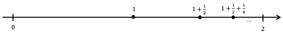
Before we can add infinitely many numbers together we must find a way to give meaning to the idea of adding infinitely many numbers. To do this, we examine an infinite sum by thinking of it as a sequence of finite partial sums.
Since each partial sum is located at the midpoint between the previous partial sum and \(2\text{,}\) it is reasonable to suppose that these sums tend to the number 2. Indeed, you have probably seen an expression such as
justified by a similar argument. Of course, relying on pictures is fine if we are satisfied with intuition. However, to establish rigor we cannot rely on pictures or such nebulous words as “approaches.”
No doubt you are wondering “What’s wrong with the word ‘approaches’? It seems clear enough to me.” This is often a sticking point. But if we think carefully about what we mean by the word “approach” we see that there is an implicit assumption that will cause us some difficulties later if we don’t expose it.
To see this consider the sequence \(\left(1,\frac12,\frac13,\frac14,\ldots\right)\text{.}\) Clearly it “approaches” zero, right? But, doesn’t it also “approach” \(-1?\) It does, in the sense that each term gets closer to \(-1\) than the one previous. But it also “approaches” \(-2\text{,}\)\(-3\text{,}\) or even \(-1000\) in the same sense. That’s the problem with the word “approaches.” It just says that at each step we’re closer to something than we were in the previous step. It does not tell us that we are actually getting close. Since the moon moves in an elliptical orbit about the earth for part of each month it is “approaching” the earth. The moon gets closer to the earth but, thankfully, it does not get close to the earth.
The implicit assumption we alluded to earlier is this: When we say that the sequence \(\left(\frac1n\right)_{n=1}^\infty\) “approaches” zero we mean that it is getting close not closer. Ordinarily this kind of vagueness in our language is pretty innocuous. When we say “approaches” in casual conversation we can usually tell from the context of the conversation whether we mean “getting close to” or “getting closer to.” But when speaking mathematically we need to be more careful, more explicit, in the language we use.
So how can we change the language we use so that this ambiguity is eliminated? We start by recognizing, rigorously, what we mean when we say that a sequence converges to zero. For example, you would probably want to say that the sequence \(\left(1,\frac{1}{2},\frac{1}{3},\frac{1}{4},\,\ldots\right)=\left(
\frac{1}{n}\right)_{n=1}^\infty\) converges to zero. Is there a way to give this meaning without relying on pictures or intuition?
One way would be to say that we can make \(\frac{1}{n}\) as close to zero as we wish, provided we make \(n\) large enough. But even this needs to be made more specific. For example, we can get \(\frac{1}{n}\) to within a distance of \(0.1\) of \(0\) provided we make \(n>10\text{,}\) we can get \(\frac{1}{n}\) to within a distance of \(0.01\) of \(0\) provided we make \(n>100\text{,}\) etc. After a few such examples it is apparent that given any arbitrary distance \(\eps>0\text{,}\) we can get \(\frac{1}{n}\) to within \(\eps\) of \(0\) provided we make \(n>\frac{1}{\eps}\text{.}\) This leads to the following definition.
Definition6.1.1.Convergence to Zero of a Sequence.
Let \(\left(s_n\right)=\left(s_1,s_2,s_3,\ldots\right)\) be a sequence of real numbers. We say that \(\left(\boldsymbol{s}_{\boldsymbol{n}}\right)\) converges to 0 and write
This definition is the formal version of the idea we just talked about. Given an arbitrary distance \(\eps\text{,}\) we must be able to find a specific number \(N\) such that \(s_n\) is within \(\eps\) of \(0\text{,}\) whenever \(n>N\text{.}\) The \(N\) is the answer to the question, how large is “large enough” to put \(s_n\) this close to \(0\text{.}\)
Even though we didn’t need it in the example \(\left(\frac{1}{n}\right)\text{,}\) the absolute value appears in the definition because we need to make the distance from \(s_n\) to 0 smaller than \(\eps\text{.}\) Without the absolute value in the definition, we would be able to “prove” such outrageous statements as \(\limitt{n}{\infty}{-n}=0\text{,}\) which we obviously don’t want.
The statement \(|s_n|\lt \eps\) can also be written as \(-\eps\lt s_n\lt \eps\) or \(s_n\in\left(-\eps,\eps\right)\text{.}\) (See the Problem 6.1.2 below.) Any one of these equivalent formulations can be used to prove convergence. Depending on the application, one of these may be more advantageous to use than the others.
Any time an \(N\) can be found that works for a particular \(\eps\text{,}\) any number \(M>N\) will work for that \(\eps\) as well, since if \(n>M\) then \(n>N\text{.}\)
Let \(\eps>0\) be given. Let \(N=\frac{1}{\eps}\text{.}\) If \(n>N\text{,}\) then \(n>\frac{1}{\eps}\) and so \(\abs{\frac{1}{n}}=\frac{1}{n}\lt \eps\text{.}\) Hence by definition, \(\limitt{n}{\infty}{\frac{1}{n}}=0\text{.}\)
Notice that this proof is rigorous and makes no reference to vague notions such as “getting smaller” or “approaching infinity.” It has three components:
provide the challenge of a distance \(\eps>0\text{,}\)
There is also no explanation about where \(N\) came from. While it is true that this choice of \(N\) is not surprising in light of the “scrapwork” we did before the definition, the motivation for how we got it is not in the formal proof nor is it required. In fact, such scrapwork is typically not included in a formal proof. For example, consider the following.
Let \(\eps>0\text{.}\) Let \(N=\frac{1}{\eps}\text{.}\) If \(n>N\text{,}\) then \(n>\frac{1}{\eps}\) and \(\frac{1}{n}\lt \eps\text{.}\) Thus \(\abs{\frac{\sin(n)}{n}}\leq\frac{1}{n}\lt \eps\text{.}\) Hence by definition, \(\limitt{n}{\infty}{\frac{\sin n}{n}}=0\text{.}\)
Notice that the \(N\) came out of nowhere, but you can probably see the thought process that went into this choice: We needed to use the inequality \(\abs{\sin n}\leq 1\text{.}\) Again this scrapwork is not part of the formal proof, but it is typically necessary for finding what \(N\) should be. You might be able to do the next problem without doing any scrapwork first, but don’t hesitate to do scrapwork if you need it.
Given an \(\eps>0\text{,}\) we need to see how large to make \(n\) in order to guarantee that \(|\frac{n+4}{n^2+1}|\lt \eps\text{.}\) First notice that \(\frac{n+4}{n^2+1}\lt \frac{n+4}{n^2}\text{.}\) Also, notice that if \(n>4\text{,}\) then \(n+4\lt n+n=2n\text{.}\) So as long as \(n>4\text{,}\) we have \(\frac{n+4}{n^2+1}\lt \frac{n+4}{n^2}\lt \frac{2n}{n^2}=\frac{2}{n}\text{.}\) We can make this less than \(\eps\) if we make \(n>\frac{2}{\eps}\text{.}\) This means we need to make \(n>4\) and \(n>\frac{2}{\eps}\text{,}\) simultaneously. These can be done if we let \(N\) be the maximum of these two numbers. This sort of thing comes up regularly, so the notation \(N=\max\left(4,\frac{2}{\eps}\right)\) was developed to mean the maximum of these two numbers. Notice that if \(N=\max\left(4, \frac{2}{\eps}\right)\) then \(N\geq 4\) and \(N\geq\frac{2}{\eps}\text{.}\) We’re now ready for the formal proof.
Let \(\eps>0\text{.}\) Let \(N=\max\left(4,\frac{2}{\eps}\right)\text{.}\) If \(n>N\text{,}\) then \(n>4\) and \(n>\frac{2}{\eps}\text{.}\) Thus we have \(n>4\) and \(\frac{2}{n}\lt \eps\text{.}\) Therefore
Again we emphasize that the scrapwork is not explicitly a part of the formal proof. However, if you look carefully, you can always find the scrapwork in the formal proof.
We can negate Definition 6.1.1 to prove that a particular sequence does not converge to zero. Before we look at an example, let’s analyze what it means for a sequence \(\left(s_n\right)\) to not converge to zero.
Converging to zero means that any time a distance \(\eps>0\) is given, we must be able to respond with a number \(N\) such that \(|s_n|\lt \eps\) for every \(n>N\text{.}\) To have this not happen, we must be able to find some \(\eps>0\) such that no choice of \(N\) will work. Of course, if we find such an \(\eps\text{,}\) then any smaller value will also fail to have such an \(N\text{,}\) but we only need one.
If you stare at the example long enough, you see that any \(\eps\) with \(0\lt \eps\leq 2\) will cause problems. For the sake of specificity (rigor) we will let \(\eps=2\text{.}\)
Also let \(N\in\RR\) be any real number. If we let \(k\) be any non–negative integer with \(k>\frac{N}{2}\text{,}\) then \(n=2k>N\text{,}\) but \(|1+(-1)^n|=2\text{.}\) Thus no choice of \(N\) will satisfy the conditions of the definition for this \(\eps\text{,}\) (namely that \(|1+(-1)^n|\lt 2\) for all \(n>N\)) and so \(\limit{n}{\infty}{\left(1+(-1)^n\right)}\neq 0\text{.}\)
Now that we have a handle on how to rigorously prove that a sequence converges to zero, let’s generalize this to a formal definition for a sequence converging to something else. Basically, we want to say that a sequence \(\left(s_n\right)\) converges to a real number \(s\text{,}\) provided the difference \(\left(s_n-s\right)\) converges to zero. This leads to the following definition:
Let \(\left(s_n\right)=\left(s_1,s_2,s_3,\ldots\right)\) be a sequence of real numbers and let \(s\) be a real number. We say that \(\left(\boldsymbol{s}_{\boldsymbol{n}}\right)\) converges to \(\boldsymbol{s}\) and write \(\limitt{n}{\infty}{s_n}=s\) provided for any \(\eps>0\text{,}\) there is a real number \(N\) such that if \(n>N\text{,}\) then \(|s_n-s|\lt \eps\text{.}\)
Again notice that this says that we can make \(s_n\) as close to \(s\) as we wish (within \(\eps\)) by making \(n\) large enough (\(>N)\text{.}\) As before, this definition makes these notions very specific.
Let \(\eps>0\text{.}\) Let \(N=\frac{100}{\eps}\text{.}\) If \(n>N\text{,}\) then \(n>\frac{100}{\eps}\) and so \(\frac{100}{n}\lt \eps\text{.}\) Hence
Notice again that the scrapwork is not part of the formal proof and the author of a proof is not obligated to explain where the choice of \(N\) came from (although the thought process can usually be seen in the formal proof). The formal proof contains only these requisite three parts:
provide the challenge of an arbitrary \(\eps>0\text{,}\)
Also notice that given a specific sequence such as \(\left(\frac{n}{n+100}\right)\text{,}\) the definition does not indicate what the limit would be if in fact, it exists. Once an educated guess is made the definition only verifies that this intuition is correct.
This leads to the following question: If intuition is needed to determine what a limit of a sequence should be, then what is the purpose of this relatively non–intuitive, complicated definition?
Remember that when these rigorous formulations were developed, intuitive notions of convergence were already in place and had been used with great success. But the arguments based on them could not be fully justified. This definition was developed to address the foundational issues, not to help us compute limits.
Could our intuitions be verified in a concrete fashion that was above reproach? This was the purpose of this non-intuitive definition. It was to be used to verify that our intuition was, in fact, correct and do so in a very prescribed manner. For example, if \(b>0\) is a fixed number, then you would probably say as \(n\) approaches infinity, \(b^{\left(\frac{1}{n}\right)}\) approaches \(b^0=1\text{.}\) After all, we did already prove that \(\limit{n}{\infty}{\frac{1}{n}}=0\text{.}\) We should be able to back up this intuition with our rigorous definition.
Choose \(\eps=1\) and use the fact that \(\abs{a-(-1)^n}\lt 1\) is equivalent to \(\left(-1\right)^n-1\lt a\lt \left(-1\right)^n+1\) to show that no choice of \(N\) will work for this \(\eps\text{.}\)
Prove that if \(\limit{n}{\infty}{s_n}=s\) then \(\limit{n}{\infty}{\abs{s_n}}=\abs{s}\text{.}\) Prove that the converse is true when \(s=0\text{,}\) but it is not necessarily true otherwise.
Let \(\left(s_n\right)\) and \(\left(t_n\right)\) be sequences with \(s_n\leq t_n,\forall\ n\text{.}\) Suppose \(\limit{n}{\infty}{s_n}=s\) and \(\limit{n}{\infty}{t_n}=t\text{.}\) Prove \(s\leq t\text{.}\)
Prove that if a sequence converges, then its limit is unique. That is, prove that if \(\limit{n}{\infty}{s_n}=s\) and \(\limit{n}{\infty}{s_n}=t\text{,}\) then \(s=t\text{.}\)
As you saw in the previous section the formal definition of the convergence of a sequence is meant to capture rigorously our intuitive understanding of convergence. However, the definition itself is an unwieldy tool. If only there were some way to be rigorous without having to run back to the definition each time. Fortunately, there is a way. If we can use the definition to prove some general rules about limits then we could use these rules whenever they apply and be assured that everything was still rigorous. A number of these should look familiar from Calculus.
We often state this theorem informally as “the limit of a sum is the sum of the limits.” However, to be absolutely precise, what it says is that if we already know that two sequences converge, then the sequence formed by summing their corresponding terms will also converge and in fact, it will converge to the sum of those individual limits.
We’ll provide the scrapwork and leave the formal write–up to you in Problem 6.2.5. Be sure you justify every step. Also, note the role of the triangle inequality in the proof.
If we let \(\eps>0\text{,}\) then we want to find \(N\) such that if \(n>N\text{,}\) then \(\abs{\left(a_n+b_n\right)-\left(a+b\right)}\lt \eps\text{.}\) Since we know that \(\limit{n}{\infty}{a_n}=a\) and \(\limit{n}{\infty}{b_n}=b\text{,}\) we can make \(\abs{a_n-a}\) and \(\abs{b_n-b}\) as small as we wish, provided we make \(n\) large enough. Let’s look closely at our goal to see if we can close the gap between what we know and what we want. We know, by the triangle inequality, that
Fortunately, we can do that as the definitions of \(\limit{n}{\infty}{a_n}=a\) and \(\limit{n}{\infty}{b_n}=b\) allow us to make \(\abs{a_n-a}\) and \(\abs{b_n-b}\) arbitrarily small.
Specifically, since \(\limit{n}{\infty}{a_n}=a\text{,}\) there exists an \(N_1\) such that if \(n>N_1\) then \(\abs{a_n-a}\lt \frac{\eps}{2}\text{.}\) Also since \(\limit{n}{\infty}{b_n}=b\text{,}\) there exists an \(N_2\) such that if \(n>N_2\) then \(\abs{b_n-b}\lt
\frac{\eps}{2}\text{.}\) Since we want both of these to occur, it makes sense to let \(N=\)max\(\left(N_1,N_2\right)\text{.}\) This should be the \(N\) that we seek.
SCRAPWORK: Given \(\eps>0\text{,}\) we want \(N\) so that if \(n>N\text{,}\) then \(\abs{a_n b_n-a b}\lt \eps\text{.}\) One of the standard tricks in analysis is to “uncancel.” In this case we will subtract and add a convenient term. Normally these would “cancel out,” which is why we say that we will uncancel to put them back in. You already saw an example of this in proving the Reverse Triangle Inequality (Problem 6.2.3). In the present case, consider
We can make this whole thing less than \(\eps\text{,}\) provided we make each term in the sum less than \(\frac{\eps}{2}\text{.}\) We can make \(\big|b\big|\big|a_n-a\big|\lt \frac{\eps}{2}\) if we make \(\big|a_n-a\big|\lt \frac{\eps}{2|b|}\text{.}\)
We could handle this as a separate case or we can do the following “slick trick.” Notice that we can add one more line to the above string of inequalities:
Making \(\abs{a_n}\abs{b_n-b}\lt \frac{\eps}{2}\) requires a bit more finesse. At first glance, one would be tempted to try and make \(\abs{b_n-b}\lt \frac{\eps}{2|a_n|}\text{.}\) Even if we ignore the fact that we could be dividing by zero (which we could handle), we have a bigger problem. According to the definition of \(\limitt{n}{\infty}{b_n}=b\text{,}\) we can make \(\abs{b_n-b}\) smaller than any given fixed positive number, as long as we make \(n\) large enough (larger than some \(N\) which goes with a given epsilon). Unfortunately, \(\frac{\eps}{2|a_n|}\) is not fixed as it has the variable \(n\) in it; there is no reason to believe that a single \(N\) will work with all possible values of \(n\) simultaneously. To handle this impasse, we need the following:
We know that there exists \(N\) such that if \(n>N\text{,}\) then \(\abs{a_n-a}\lt 1\text{.}\) Let \(B=\)max\(\left(\abs{a_1},\abs{a_2},\ldots,\abs{a_{\lceil{N}\rceil}},\abs{a}+1\right)\text{,}\) where \(\lceil{N}\rceil\) represents the smallest integer greater than or equal to \(N\text{.}\)
Consider \(\big|\frac{1}{b_n}-\frac{1}{b}\big|=\frac{|b-b_n|}{|b_n||b|}\text{.}\) We are faced with the same dilemma we had when we were proving Theorem 6.2.6; we need to get \(\big|\frac{1}{b_n}\big|\) bounded above. This means we need to get \(\abs{b_n}\) bounded away from zero (at least for large enough \(n\)).
This can be done as follows. Since \(b\neq 0\text{,}\) then \(\frac{|b|}{2}>0\text{.}\) Thus, by the definition of \(\limit{n}{\infty}{b_n}=b\) there exists \(N_1\) such that if \(n>N_1\text{,}\) then \(\abs{b}-\abs{b_n}\leq\big|b-b_n\big|\lt \frac{\abs{b}}{2}\text{.}\) Thus when \(n>N_1\text{,}\)\(\frac{\abs{b}}{2}\lt \abs{b_n}\) and so \(\frac{1}{\abs{b_n}}\lt \frac{2}{\abs{b}}\text{.}\) This says that for \(n>N_1\text{,}\)\(\frac{\abs{b-b_n}}{\abs{b_n}\abs{b}}\lt \frac{2}{\abs{b}^2}\abs{b-b_n}\text{.}\) We should be able to make this smaller than a given \(\eps>0\text{,}\) provided we make \(n\) large enough.
The results of Problem 6.2.1, Theorem 6.2.4, Theorem 6.2.6, and Theorem 6.2.12 allow us to find the limits of complicated sequences and then rigorously verify that these are in fact, the correct limits without resorting to the definition of a limit.
Let \(\left(r_n\right),\left(s_n\right)\text{,}\) and \(\left(t_n\right)\) be sequences of real numbers with \(r_n\leq s_n\leq t_n,\forall\) positive integers \(n\text{.}\) Suppose \(\limit{n}{\infty}{r_n}=s=\limit{n}{\infty}{t_n}\text{.}\) Then \(\left(s_n\right)\) must converge and \(\limit{n}{\infty}{s_n}=s\text{.}\)
The Squeeze Theorem is true even if \(r_n\leq s_n\leq
t_n\) only holds for sufficiently large \(n\text{;}\) i.e., for \(n\) larger than some fixed \(N_0\text{.}\) This is true because when you find an \(N_1\) that works in the original proof, this can be modified by choosing \(N=\)max\(\left(N_0,N_1\right)\text{.}\) Also note that this theorem really says two things:
Notice that \(0\leq\frac{n+1}{n^2}\leq\frac{n+n}{n^2}=\frac{2}{n}\text{.}\) Since \(\limit{n}{\infty}{0}=0=\limit{n}{\infty}{\frac{2}{n}}\text{,}\) then by the Squeeze Theorem, \(\limit{n}{\infty}{\frac{n+1}{n^2}}=0\text{.}\)
This is incorrect in form because it presumes that \(\limitt{n}{\infty}{\frac{n+1}{n^2}}\) exists, which we don’t yet know. If we knew that the limit existed to begin with, then this would be fine. The Squeeze Theorem proves that the limit does in fact exist, but it must be so stated.
Choose \(R\) with \(L\lt R\lt 1\text{.}\) By the Problem 6.1.18, \(\exists\)\(N\) such that if \(n>N\text{,}\) then \(\frac{s_{n+1}}{s_n}\lt R\text{.}\) Let \(n_0>N\) be fixed and show \(s_{n_0+k}\lt R^ks_{n_0}\text{.}\) Conclude that \(\limit{k}{\infty}{s_{n_0+k}}=0\) and let \(n=n_0+k\text{.}\)
The general theorems we have seen in this section will allow us to rigorously explore convergence of power series in the next chapter without appealing directly to the definitions. However there will still be times when we will need to apply the definition directly.
In Theorem 4.2.3 we saw that there is a rearrangment of the alternating Harmonic series which diverges to \(\infty\) or \(-\infty\text{.}\) In that section we did not fuss over any formal notions of divergence. We assumed instead that you are already familiar with the concept of divergence, probably from taking Calculus in the past.
However we are now in the process of building precise, formal definitions for the concepts we will be using so we define the divergence of a sequence as follows.
It may seem unnecessarily pedantic of us to insist on formally stating such an obvious definition. After all “converge” and “diverge” are opposites in ordinary English. Why wouldn’t they be mathematically opposite too? Why do we have to go to the trouble of formally defining both of them? Since they are opposites defining one implicitly defines the other doesn’t it?
One way to answer that criticism is to state that in mathematics we always work from precisely stated definitions and tightly reasoned logical arguments.
One reason for providing formal definitions of both convergence and divergence is that in mathematics we frequently co-opt words from natural languages like English and imbue them with mathematical meaning that is only tangentially related to the original English definition. When we take two such words which happen to be opposites in English and give them mathematical meanings which are not opposites it can be very confusing, especially at first.
This is what happened with the words “open” and “closed.” These are opposites in English: “not open” is “closed,” “not closed” is “open,” and there is nothing which is both open and closed. But recall that an open interval on the real line, \((a,b)\text{,}\) is one that does not include either of its endpoints while a closed interval, \([a,b]\text{,}\) is one that includes both of them.
These may seem like opposites at first but they are not. To see this observe that the interval \((a,b]\) is neither open nor closed since it only contains one of its endpoints. If “open” and “closed” were mathematically opposite then every interval would be either open or closed.
Mathematicians have learned to be extremely careful about this sort of thing. In the case of convergence and divergence of a series, even though these words are actually opposites mathematically (every sequence either converges or diverges and no sequence converges and diverges) it is better to say this explicitly so there can be no confusion.
A sequence \(\left(a_n\right)_{n=1}^\infty\) can only converge to a real number, \(a\text{,}\) in one way: by getting arbitrarily close to \(a\text{.}\) However there are several ways a sequence might diverge.
Consider the sequence, \(\left(n\right)_{n=1}^\infty\text{.}\) This clearly diverges by getting larger and larger \(\ldots\) Ooops! Let’s be careful. The sequence \(\left(1-\frac1n\right)_{n=1}^\infty\) gets larger and larger too, but it converges. What we meant to say was that the terms of the sequence \(\left(n\right)_{n=1}^\infty\) become arbitrarily large as \(n\) increases.
To show divergence we must show that the sequence satisfies the negation of the definition of convergence. That is, we must show that for every \(r\in\RR\) there is an \(\eps>0\) such that for every \(N\in\RR\text{,}\) there is an \(n>N\) with \(\left|n-r\right|\ge\eps\text{.}\)
To prove that the sequence diverges let \(N\in \RR \) and \(r\in \RR \) be given. Take \(\eps=1\text{.}\) Let \(N_0\) be the smallest positive integer which is greater than \(r\text{.}\) Finally take \(n\) to be greater than \(N\text{,}\)\(N_0\) and \(r+2\text{.}\)
The fact that \(\left(n\right)_{n=1}^\infty \) diverges can be proved by simpler means than we used in Example 6.3.2. For example, we could use Lemma 6.2.7.
Since these (much) simpler methods were available to us why do you suppose we chose to present a tedious and difficult proof based on the negation of Definition 6.1.10?
The fact is that mathematical definitions are not primarily intended to serve as tools for problem solving (theorem proving). The chief purpose of a definition is to clarify our ideas and make them precise. Lemmas and theorems (the solutions of problems) are then built up logically from definitions. And they provide the tools we need to solve more difficult, or abstract problems (prove lemmas and theorems). Recall that in Section 1.3 we empasized that “A problem, once solved, becomes a tool for solving subsequent problems!” Taken together Example 6.3.2, Problem 6.3.3, Definition 6.3.4, and Problem 6.3.6 are intended to illustrate the robustness of this approach to mathematics.
A sequence, \(\left(a_n\right)_{n=1}^\infty\text{,}\) diverges to positive infinity if for every real number \(r\text{,}\) there is a real number \(N\) such that \(n>N\imp a_n>r\text{.}\)
A sequence, \(\left(a_n\right)_{n=1}^\infty\text{,}\) diverges to negative infinity if for every real number \(r\text{,}\) there is a real number \(N\) such that \(n>N\imp a_n\lt r\text{.}\)
Speaking informally, Definition 6.3.4 says that \(\left(a_n\right)_{n=1}^\infty{}\) diverges to infinity if it becomes arbitrarily large in either the positive or the negative direction as \(n\) increases.
However, strictly speaking this is an abuse of notation since the symbol \(\infty\) does not represent a real number. This notation can be very problematic since it looks so much like the notation we use to denote convergence: \(\limit{n}{\infty}{a_n}=a\text{.}\)
Nevertheless, the notation is appropriate because divergence to infinity is “nice” divergence in the sense that it shares many of the properties of convergence, as the next problem shows.
Because divergence to positive or negative infinity shares some of the properties of convergence it is easy to get careless with it. Remember that even though we write \(\limit{n}{\infty}{a_n}=\infty\) this is still a divergent sequence in the sense that \(\limit{n}{\infty}{a_n}\) does not exist. The symbol \(\infty\) does not represent a real number. This is just a convenient notational shorthand telling us that the sequence diverges by becoming arbitrarily large.
Suppose that \(\left(a_n\right)_{n=1}^\infty\) diverges but not to infinity and that \(\alpha\) is a real number. What conditions on \(\alpha\) will guarantee that: