Chapter5Joseph Fourier: The Man Who Broke Calculus
Section5.1Joseph Fourier and His Series
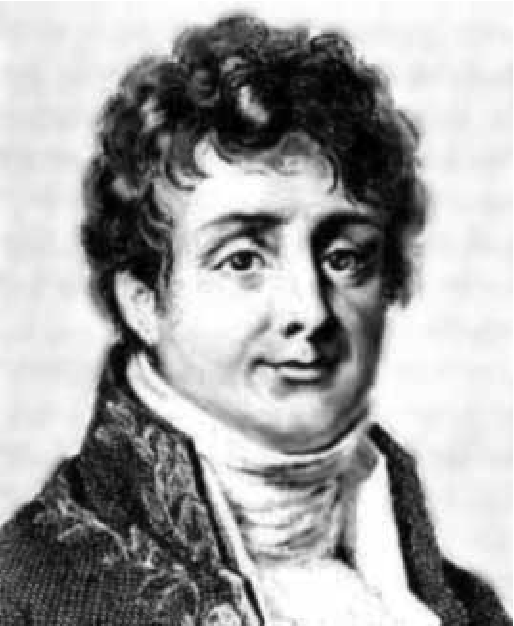
Applying mathematics to physical problems such as heat flow in a solid body drew much attention in the latter part of the 1700’s and the early part of the 1800’s. One of the people to attack the heat flow problem was Jean Baptiste Joseph Fourier (1768–1839).
Fourier submitted a manuscript on the subject, Sur la propagation de la chaleur (On the Propagation of Heat), to the Institut National des Sciences et des Arts in 1807. These ideas were subsequently published in La theorie analytique de la chaleur (The Analytic Theory of Heat (1822)).
To examine Fourier’s ideas, consider the example of a thin wire of length one, which is perfectly insulated and whose endpoints are held at a fixed temperature of zero. Given an initial temperature distribution in the wire, the problem is to monitor the temperature of the wire at any point \(x\) and at any time \(t\text{.}\) Specifically, if we let \(u(x,t)\) denote the temperature of the wire at point \(x\in[0,1]\) at time \(t\geq 0\text{,}\) then it can be shown that \(u\) must satisfy the one-dimensional heat equation \(\rho^2\frac{\partial^2u}{\partial x^2}=\frac{\partial
u}{\partial t}\text{,}\) where \(\rho^2\) is a positive constant known as the thermal diffusivity. If the initial temperature distribution is given by the function \(f(x)\text{,}\) then the \(u\) we are seeking must satisfy all of the following.
To do this, Fourier employed what is now referred to as the method of separation of variables. Specifically, Fourier looked for solutions of the form \(u(x,t)=X(x)T(t)\text{;}\) that is, solutions where the \(x\)–part can be separated from the \(t\)-part. Assuming that \(u\) has this form, we get \(\frac{\partial^2u}{\partial x^2}=X^{\prime\prime}T\) and \(\frac{\partial u}{\partial t}=X\,T^{\prime}\text{.}\) Substituting these into equation (5.1.1) we obtain
Show that \(T=Ce^{\rho^2kt}\) satisfies the equation \(T^\prime=\rho^2k T\text{,}\) where \(C\) is an arbitrary constant. Use the physics of the problem to show that if \(u\) is not constantly zero, then \(k\lt 0\text{.}\)
Show that \(X=A\sin\left(px\right)+B\cos\left(px\right)\) satisfies the equation \(X^{\prime\prime}=-p^2X\text{,}\) where \(A\) and \(B\) are arbitrary constants. Use the boundary conditions \(u(0,t)=u(1,t)=0\text{,}\)\(\forall\)\(t\geq 0\) to show that \(B=0\) and \(A\sin p=0\text{.}\) Conclude that if \(u\) is not constantly zero, then \(p=n\pi\text{,}\) where \(n\) is any integer.
All that is left is to have \(u\) satisfy the initial condition \(u(x,0)=f(x)\text{,}\)\(\forall\,x\in[\,0,1]\text{.}\) That is, we need to find coefficients \(A_n\text{,}\) such that
The idea of representing a function as a series of sine waves was proposed by Daniel Bernoulli in 1753 while examining the problem of modeling a vibrating string. Unfortunately for Bernoulli, he didn’t know how to compute the coefficients in such a series representation. What distinguished Fourier was that he developed a technique to compute these coefficients. The key is the result of the following problem.
Armed with the result from Problem 5.1.5, Fourier could compute the coefficients \(A_n\) in the series representation \(f(x)=\sum_{n=1}^\infty A_n \sin\left(n\pi x\right)\) in the following manner. Since we are trying to find \(A_n\) for a particular (albeit general) \(n\text{,}\) we will temporarily change the index in the summation from \(n\) to \(j\text{.}\) With this in mind, consider
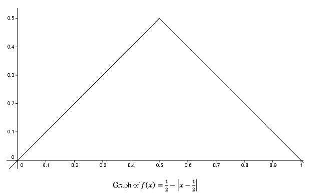
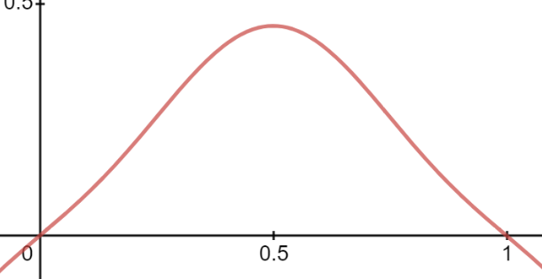
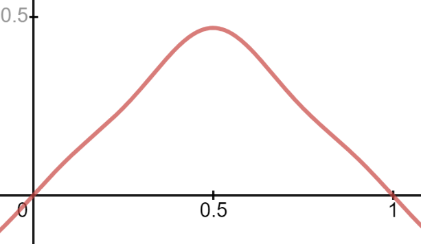
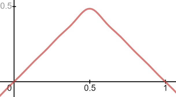
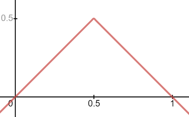
be the \(Nth\) partial sum of the series. The sketches below display the graphs of \(S_N\) when \(N=1\text{,}\)\(N=2\text{,}\)\(N=5\text{,}\) and \(N=50\text{.}\)
As you can see, as we add more terms to \(S_N\) its graph looks more and more like the original function \(f(x)=\frac{1}{2}-\abs{x-\frac{1}{2}}\text{.}\) This would seem to be strong evidence that series converges to the function and therefore
Recall, that when we represented a function as a power series, we freely differentiated and integrated the series term by term as though it was a polynomial. Let’s do the same with this Fourier series.
Let \(C_N(x)=\frac{4}{\pi}\sum_{k=0}^N\frac{\left(-1\right)^k}{\left(2k+1\right)}
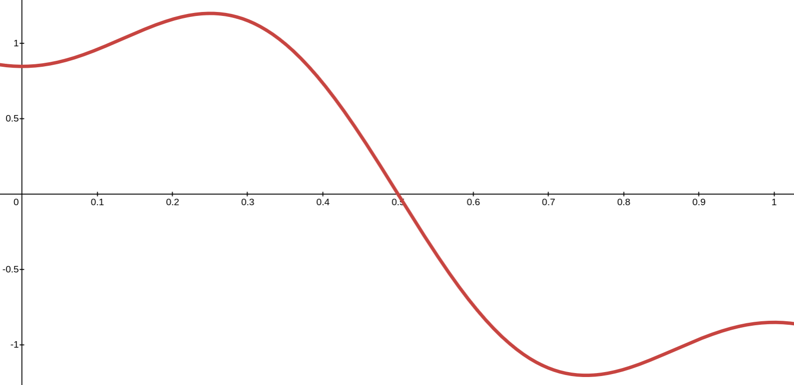
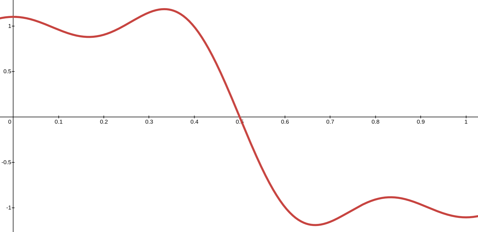
\cos\left(\left(2k+1\right)\pi x\right)\) be the \(Nth\) partial sum of this Fourier cosine series. The sketches below display the graphs of \(C_N\) when \(N=1\text{,}\)\(N=2\text{,}\)\(N=5\text{,}\) and \(N=50\text{.}\)
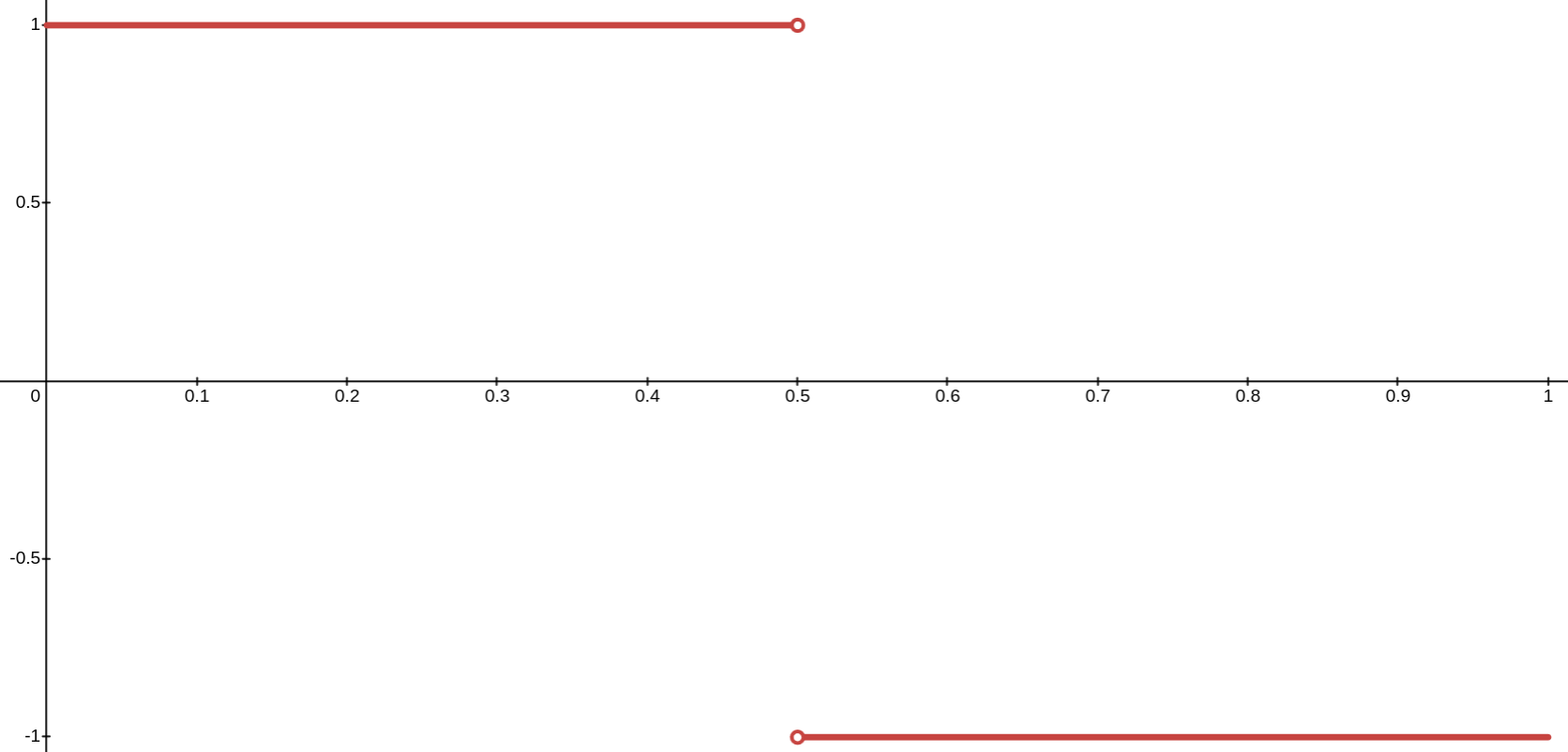
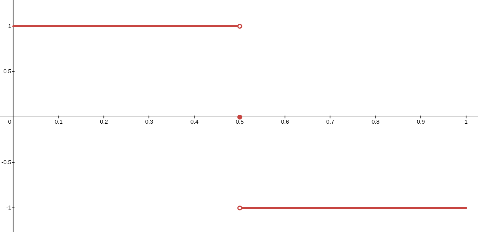
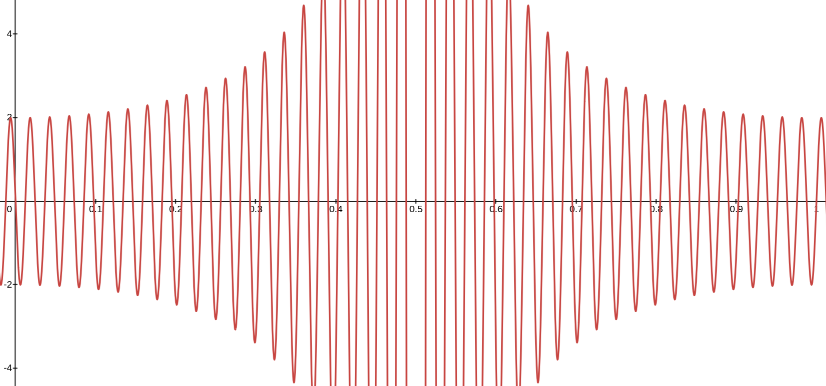
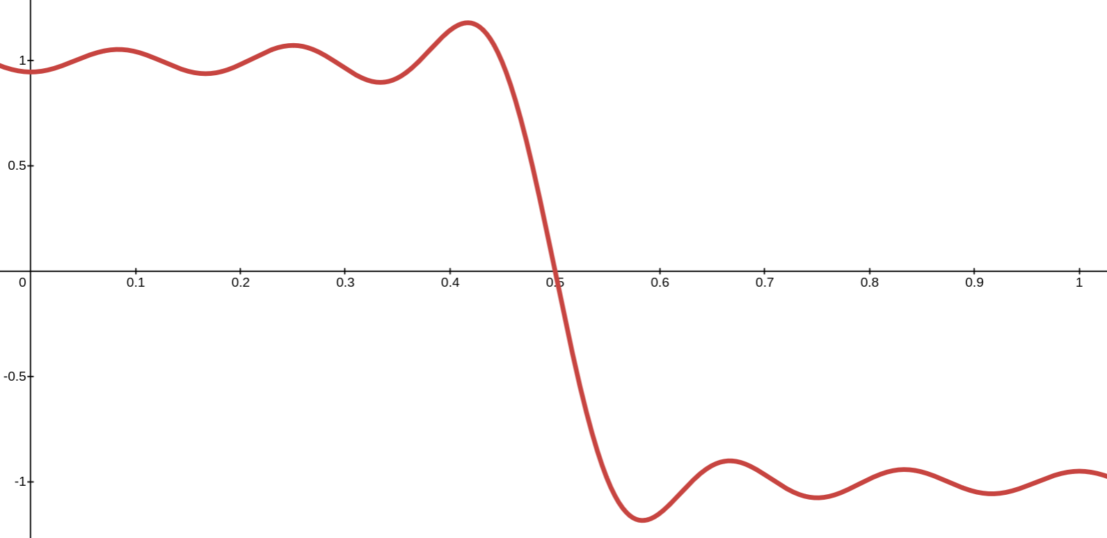
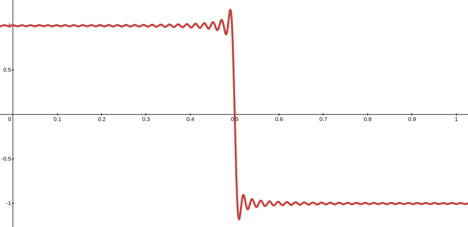
In fact, if we were to graph the series \(\frac{4}{\pi}\sum_{k=0}^\infty\frac{\left(-1\right)^k}{\left(2k+1\right)}\) cos\(\left(\left(2k+1\right)\pi x\right)\text{,}\) we would obtain the following graph:
Notice that this agrees with the graph of \(f^\prime\text{,}\) except that \(f^\prime\) didn’t exist at \(x=\frac{1}{2}\text{,}\) and this series takes on the value \(0\) at \(x=\frac{1}{2}\text{.}\) Notice also, that every partial sum of this series is continuous, since it is a finite combination of continuous cosine functions. This agrees with what you learned in Calculus, the (finite) sum of continuous functions is always continuous. In the 1700s it was assumed (falsely) that this could be extended to infinite series, because every time a power series converged to a function, that function happened to be continuous. This never failed for power series, so this example was a bit disconcerting as it is an example of the sum of infinitely many continuous functions which is, in this case, discontinuous. Was it possible that there was some power series which converged to a function which was not continuous? Even if there isn’t, what is the difference between power series and this Fourier series?
term–by–term as before. Given the above graph of this series, it appears that the derivative of it should be constantly 0, except at \(x=\frac{1}{2}\text{,}\) where the derivative doesn’t exist. But when we perform the differentiation term–by–term we obtain the series
term by term, this differentiated series doesn’t converge to anything at \(x=\frac{1}{4}\text{,}\) let alone converge to zero. In this case, the old Calculus rule that the derivative of a sum is the sum of the derivatives does not apply for this infinite sum, though it did apply before. As if the continuity issue wasn’t bad enough before, this was even worse. Power series were routinely differentiated and integrated term-by-term. This was part of their appeal. They were treated like “infinite polynomials.” Either there is some power series lurking that refuses to behave nicely, or there is some property that power series have that not all Fourier series have.
Fortunately, the answer to that question is, “No.” Power series are generally much more well–behaved than Fourier series. Whenever a power series converges, the function it converges to will be continuous. And, as long as one stays inside the interval of convergence, power series can be differentiated and integrated term–by–term. Power series have something going for them that your average Fourier series does not, but none of this is any more obvious to us than it was to mathematicians at the beginning of the nineteenth century. What they did (and we do) know was that relying on intuition was perilous and that rigorous formulations were needed to either justify or dismiss these intuitions. In some sense, the nineteenth century was the “morning after” the mathematical party that went on throughout the eighteenth century.
and plot \(C(x,N)\) for \(N=1,2,5,50\)\(x\in[\,0,1]\text{.}\) How does this compare to the function \(f(x)=x-\frac{1}{2}\) on \([\,0,1]\text{?}\) What if you plot it for \(x\in[\,0,2]?\)
term by term and plot various partial sums for that series on \([\,0,1]\text{.}\) How does this compare to the derivative of \(f(x)=x-\frac{1}{2}\) on that interval?
Differentiate the series you obtained in part (a) and plot various partial sums of that on \([\,0,1]\text{.}\) How does this compare to the second derivative of \(f(x)=x-\frac{1}{2}\) on that interval?