The rules for Calculus were first laid out in the 1684 paper Nova methodus pro maximis et minimis, itemque tangentibus, quae nec fractas nec irrationales, quantitates moratur, et singulare pro illi calculi genus (A New Method for Maxima and Minima as Well as Tangents, Which is Impeded Neither by Fractional Nor by Irrational Quantities, and a Remarkable Type of Calculus for This) written by Gottfried Wilhelm Leibniz (1646–1716). Leibniz started with subtraction. That is, if \(x_1\) and \(x_2\) are very close together then their difference, \(\Delta
x=x_2-x_1\text{,}\) is very small. He expanded this idea to say that if \(x_1\) and \(x_2\) are infinitely close together (but still distinct) then their difference \(\dx{ x}\text{,}\) is infinitesimally small (but not zero).
This idea is logically very suspect and Leibniz knew it. But he also knew that when he used his calculus differentialis he was getting correct answers to some very hard problems. So he persevered.
Leibniz called both \(\Delta x\) and \(\dx{ x}\) differentials (Latin for difference) because he thought of them as, essentially, the same thing. Over time it has become customary to refer to the infinitesimal \(\dx{ x}\) as a differential, and to reserve the word difference and the notation \(\Delta x\) for the finite case. This is why Calculus is often called Differential Calculus.
In his paper Leibniz gave rules for dealing with these infinitely small differentials. Specifically, given a variable quantity \(x\text{,}\)\(\dx{x}\) represented an infinitesimal change in \(x\text{.}\) Differentials are related via the slope of the tangent line to a curve. That is, if \(y=f(x)\text{,}\) then \(\dx{ y}\) and \(\dx{ x}\) are related by
\begin{equation*}
\dx{ y}=\text{ (slope of the tangent line) } \cdot \dx{ x}\text{.}
\end{equation*}
The elegant and expressive notation Leibniz invented was so useful that it has been retained through the years despite some profound changes in the underlying concepts. For example, Leibniz and his contemporaries would have viewed the symbol \(\dfdx{y}{x}\) as an actual quotient of infinitesimals, whereas today we define it via the limit concept first suggested by Newton.
Leibniz states these rules without proof: “. . . the demonstration of all this will be easy to one who is experienced in such matters . . .”. Mathematicians in Leibniz’s day would have been expected to understand intuitively that if \(c\) is a constant, then
Subsection3.1.2Leibniz’s Approach to the Product Rule
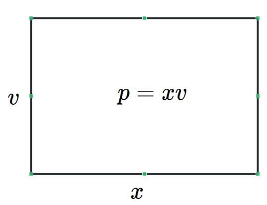
The explanation of the product rule using differentials is a bit more involved, but Leibniz expected that mathematicans would be fluent enough to derive it. The product \(p=xv\) can be thought of as the area of the following rectangle
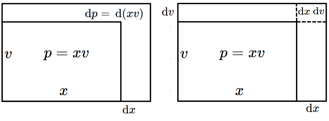
With this in mind, \(\dx{ p}=\dx{(xv)}\) can be thought of as the change in area when \(x\) is changed by \(\dx{ x}\) and \(v\) is changed by \(\dx{ v}\text{.}\) This can be seen as the L shaped region in the following drawing.
Even though \(\dx{ x}\) and \(\dx{ v}\) are infinitely small, Leibniz reasoned that \(\dx{ x}\,\dx{ v}\) is even more infinitely small (quadratically infinitely small?) compared to \(x\dx{ v}\) and \(v\dx{ x}\) and can thus be ignored leaving
You should feel some discomfort at the idea of simply tossing the product \(\dx{ x}\,\dx{ v}\) aside because it is “comparatively small.” This means you have been well trained, and have thoroughly internalized Newton’s dictum [12]: “The smallest errors may not, in mathematical matters, be scorned.” It is logically untenable to toss aside an expression just because it is small. Even less so should we be willing to ignore an expression on the grounds that it is “infinitely smaller” than another quantity which is itself “infinitely small.”
Newton and Leibniz both knew this as well as we do. But they also knew that their methods worked. They gave verifiably correct answers to problems which had, heretofore, been completely intractable. It is the mark of their genius that both men persevered in spite of the very evident difficulties their methods entailed.
Subsection3.1.3Newton’s Approach to the Product Rule
Isaac Newton’s (1643–1727) approach to Calculus — his ‘Method of Fluxions’ — depended fundamentally on motion. He conceived of variables (fluents) as changing (flowing or fluxing) in time. The rate of change of a fluent he called a fluxion. As a theoretical foundation both Leibniz’s and Newton’s approaches have fallen out of favor, although both are still universally used as a conceptual approach, a “way of thinking,” about the ideas of Calculus.
In Philosophiae naturalis principia mathematica (this is usually shortened to Principia) Newton “proved” the Product Rule as follows: Let \(x\) and \(v\) be “flowing quantites” and consider the rectangle, \(R\text{,}\) whose sides are \(x\) and \(v\text{.}\)\(R\) is also a flowing quantity and we wish to find its fluxion (derivative) at any time.
First we increment \(x\) and \(v\) by the half–increments \(\frac{\Delta
x}{2}\) and \(\frac{\Delta v}{2}\) respectively. Then the corresponding half–increment of \(R\) is
This argument is no better than Leibniz’s as it relies heavily on the number \(1/2\) to make it work. If we take any other increments in \(x\) and \(v\) whose total lengths are \(\Delta x\) and \(\Delta v\) it will simply not work. Try it and see.
In Newton’s defense, he wasn’t really trying to justify his mathematical methods in the Principia. His attention was on physics, not math, so he was really just trying to give a convincing demonstration of his methods. You may decide for yourself how convincing his demonstration is.
Notice that there is no mention of limits of difference quotients or derivatives. In fact, the term derivative was not coined until 1797, by Lagrange as we will see in Section 4.1 . In a sense, these topics were not necessary at the time, as Leibniz and Newton both assumed that the curves they dealt with had tangent lines and, in fact, Leibniz explicitly used the tangent line to relate two differential quantities. This was consistent with the thinking of the time and for the duration of this chapter we will also assume that all quantities are differentiable. As we will see later this assumption leads to difficulties.
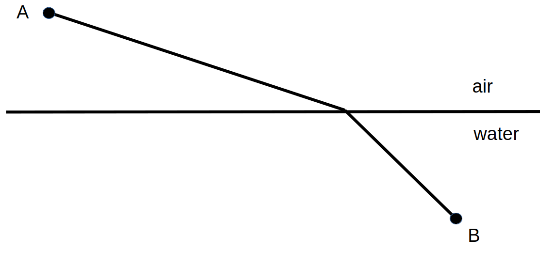
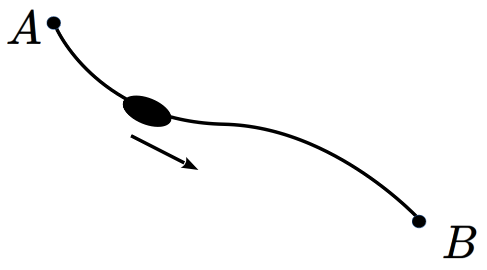
To prove the worth of his Calculus Leibniz also provided applications. As an example he derived Snell’s Law of Refraction from his Calculus rules as follows.
Given that light travels through air at a speed of \(v_a\) and travels through water at a speed of \(v_w\) the problem is to find the fastest path from point \(A\) to point \(B\text{.}\)
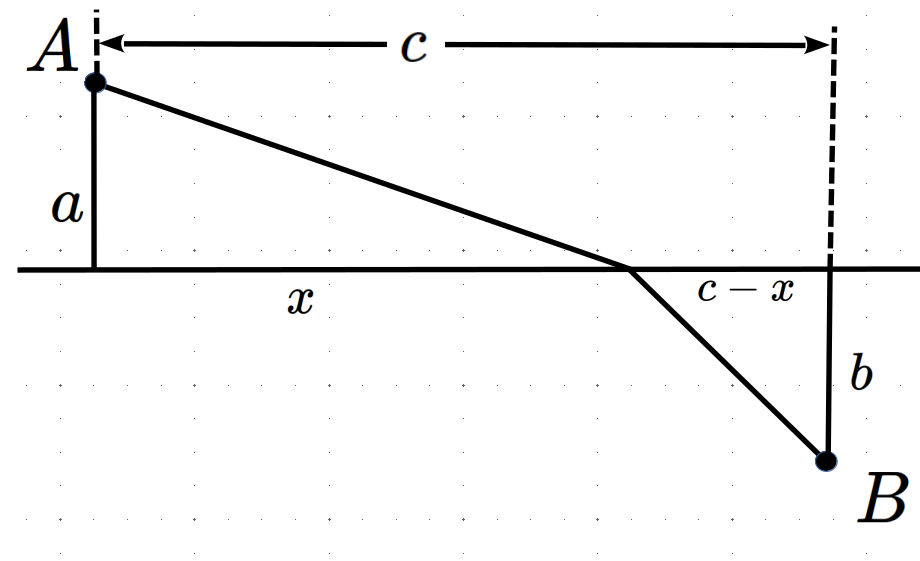
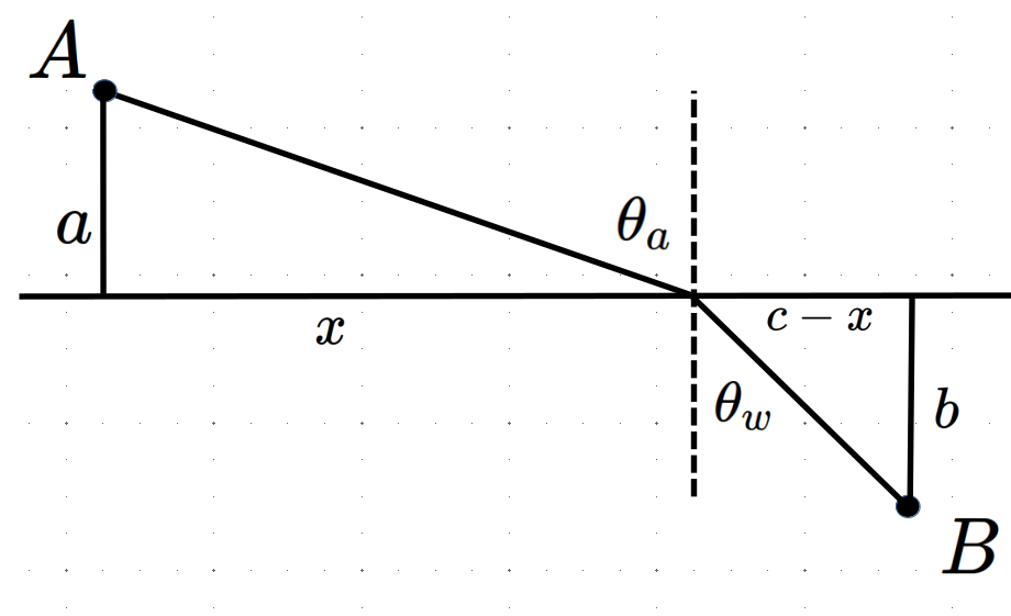
Using the fact that \(\text{ Time }=\frac{\text{Distance}}{\text{Velocity}}\) and the labeling in the picture below we can obtain a formula for the time \(T\) it takes for light to travel from \(A\) to \(B\text{.}\)
To compare 18th century and modern techniques we will consider Johann Bernoulli’s (1667–1748) solution of the Brachistochrone Problem. In 1696, Bernoulli posed and solved, the Brachistochrone problem: To find the shape of a frictionless wire joining points \(A\) and \(B\) so that the time it takes for a bead to slide down under the force of gravity is as small as possible.
Bernoulli posed this “path of fastest descent” problem to challenge the mathematicians of Europe and used his solution to demonstrate the power of Leibniz’ Calculus as well as his own ingenuity.
I, Johann Bernoulli, address the most brilliant mathematicians in the world. Nothing is more attractive to intelligent people than an honest, challenging problem, whose possible solution will bestow fame and remain as a lasting monument. Following the example set by Pascal, Fermat, etc., I hope to gain the gratitude of the whole scientific community by placing before the finest mathematicians of our time a problem which will test their methods and the strength of their intellect. If someone communicates to me the solution of the proposed problem, I shall publicly declare him worthy of praise. [13]
In addition to Johann’s, solutions were obtained from Newton, Leibniz, Johann’s brother Jacob Bernoulli, and the Marquis de l’Hopital [17]. At the time there was an ongoing and very vitriolic controversy raging over whether Newton or Leibniz had been the first to invent Calculus. As an advocate for Leibniz, Bernoulli did not believe Newton would be able to solve the problem using his fluxions. So this challenge was in part an attempt to embarrass Newton. However Newton solved it easily.
At this point in his life Newton had all but quit science and mathematics and was fully focused on his administrative duties as Master of the Mint. Due in part to rampant counterfeiting, England’s money had become severely devalued and the nation was on the verge of economic collapse. The solution was to recall all of the existing coins, melt them down, and strike new ones. As Master of the Mint this job fell to Newton [10]. As you might imagine this was a rather Herculean task. Nevertheless, according to his niece (and housekeeper):
When the problem in 1696 was sent by Bernoulli–Sir I.N. was in the midst of the hurry of the great recoinage and did not come home till four from the Tower very much tired, but did not sleep till he had solved it, which was by four in the morning.
Newton submitted his solution anonymously, presumably to avoid more controversy. Nevertheless the methods he used were so distinctively Newton’s that Bernoulli is said to have exclaimed “Tanquam ex ungue leonem.”
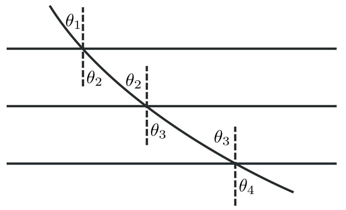
Newton’s solution was clever but it doesn’t provide any insights we’ll be interested in so we will focus on Bernoulli’s ingenious solution which starts, interestingly enough, with Snell’s Law of Refraction. He begins by considering the stratified medium in the following figure, where an object travels with velocities \(v_1, v_2, v_3, \ldots\) in the various layers.
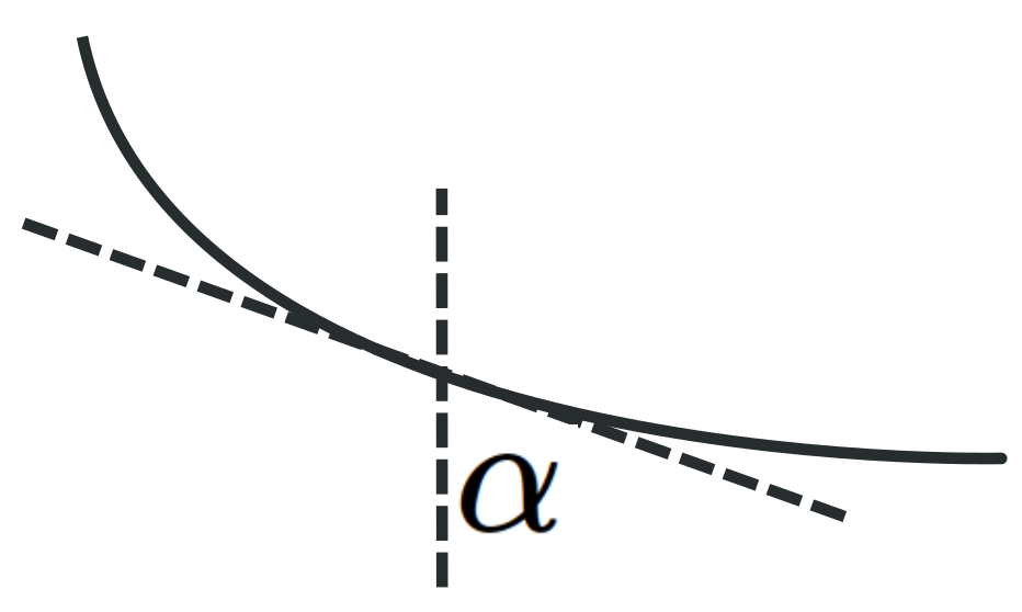
If we think of a continuously changing medium as stratified into infinitesimal layers and extend Snell’s law to an object whose speed is constantly changing, then along the fastest path, the ratio of the sine of the angle that the curve’s tangent makes with the vertical, \(\alpha\text{,}\) and the speed, \(v\text{,}\) must remain constant,
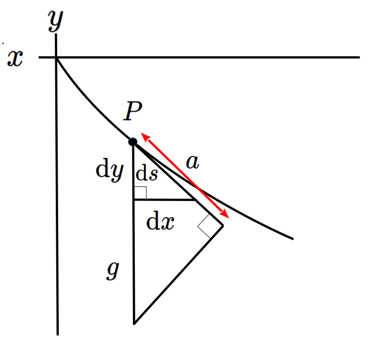
If we include the horizontal and vertical axes (with the positive \(y\)–axis pointing downward) and let \(P\) denote the position of the bead at a particular time then we have the following picture.
In Figure 3.1.15, \(s\) denotes the length that the bead has traveled down to point \(P\) (that is, the arc length of the curve from the origin to that point) and \(a\) denotes the tangential component of the acceleration due to gravity \(g\text{.}\) Since acceleration is the rate of change of velocity with respect to time we see that
By similar triangles we have \(\frac{a}{g}=\frac{\dx{ y}}{\dx{ s}}\text{.}\) As a student of Leibniz, Bernoulli would have regarded \(\frac{\dx{ y}}{\dx{ s}}\) as a fraction so
In the seventeenth, eighteenth, and even well into the nineteenth centuries, European mathematicians regarded \(\dx{ v}, \dx{ t}\text{,}\) and \(\dx{ s}\) as infinitesimally small numbers which nevertheless obey all of the usual rules of algebra. Thus they would simply rearrange equation (3.1.4), to get
Bernoulli would have interpreted this as a statement that two rectangles of height \(v\) and \(g\text{,}\) with respective widths \(\dx{ v}\) and \(\dx{ y}\) have equal area. Summing (integrating) all such rectangles we g et:
You are undoubtedly uncomfortable with the cavalier manipulation of infinitesimal quantities you’ve just witnessed, so we’ll pause for a moment now to compare a modern development of equation (3.1.5) to Bernoulli’s. As before we begin with the equation:
\begin{align*}
\frac{a}{g}\amp = \dfdx{y}{s}\\
a \amp = g\dfdx{y}{s}.
\end{align*}
Moreover, since acceleration is the derivative of velocity this is the same as:
Now observe that by the Chain Rule \(\dfdx{v}{t} =
\dfdx{v}{s}\dfdx{s}{t}\text{.}\) The physical interpretation of this formula is that velocity will depend on \(s\text{,}\) how far down the wire the bead has moved, but that the distance traveled will depend on how much time has elapsed. Therefore
In effect, in the modern formulation we have traded the simplicity and elegance of differentials for a comparatively cumbersome repeated use of the Chain Rule. No doubt you noticed when taking Calculus that in the differential notation of Leibniz, the Chain Rule looks like we are simply “canceling” a factor in the top and bottom of a fraction: \(\dfdx{y}{u}\dfdx{u}{x} = \dfdx{y}{x}\text{.}\) This is because for 18th century mathematicians, that is exactly what it was, and Leibniz designed his notation to reflect that viewpoint.
To put it another way, 18th century mathematicians wouldn’t have recognized a need for what we call the Chain Rule because this operation was a triviality for them. Just reduce the fraction. This begs the question: Why did we abandon such a clear and simple interpretation of our symbols in favor of the comparatively more cumbersome modern interpretation? This is one of the questions we will try to answer in this course.
Show that the equations \(x=\frac{\phi-\sin
\phi}{4gc^2},\,y=\frac{1-\cos \phi}{4gc^2}\) satisfy equation equation (3.1.6). Bernoulli recognized this solution to be an inverted cycloid, the curve traced by a fixed point on a circle as the circle rolls along a horizontal surface.
This illustrates the state of Calculus in the late 1600s and early 1700s; the foundations of the subject were a bit shaky but there was no denying its power.
Applied to polynomials, the rules of differential and integral Calculus are straightforward. Indeed, differentiating and integrating polynomials represent some of the easiest tasks in a Calculus course. For example, computing \(\int(7-x+x^2)\dx{
x}\) is relatively easy compared to computing \(\int\sqrt[3]{1+x^3}\dx{ x}\text{.}\) Unfortunately, not all functions can be expressed as a polynomial. For example, \(f(x)=\sin x\) cannot be since a polynomial has only finitely many roots and the sine function has infinitely many roots, namely \(\{n\pi|\,n\in\ZZ\}\text{.}\) A standard technique in the 18th century was to write such functions as an “infinite polynomial,” or what today we refer to as a power series. Unfortunately an “infinite polynomial” is a much more subtle object than a mere polynomial, which by definition is finite. For now we will not concern ourselves with these subtleties. Instead we will follow the example of our forebears and manipulate all “polynomial–like” objects (finite or infinite) as if they are polynomials.
In this section we will focus on power series centered around zero. In the next section we will look at power series centered about points other than zero.
The most advantageous way to represent a power series is using summation notation since there can be no doubt about the pattern in the terms. After all, this notation contains a formula for the general term. However, there are instances where summation notation is not practical. In these cases, it is acceptable to indicate the sum by supplying the first few terms and using ellipses (the three dots). If this is done, then enough terms must be included to make the pattern clear to the reader.
For each value of \(x\) a power series reduces to a different ordinary (numerical) series. For example, if we substitute \(x=\frac{1}{10}\) into the left side of equation (3.2.1), we obtain the (numerical) series
If these computations are valid then it must be that \(1.111\ldots=\frac{10}{9}\text{,}\) which seems weird, but you can verify it by entering \(\frac{10}{9}\) into any calculator.
which seems like nonsense. It simply can’t be true, can it? What do you think? Is \(0.999\ldots =1\) or that just nonsense? Either way it is clear that the real numbers \(\left(\RR\right) \) hide deeper mysteries than the irrationality of \(\sqrt{2}\text{.}\)
A power series representation of our function seems to work in some cases, but not in others. Obviously we are missing something important here, though it may not be clear exactly what. For now, we will continue to follow the example of our 18th century predecessors. That is, for the rest of this section we will use formal manipulations to obtain and use power series representations of various functions. Keep in mind that this is all highly suspect until we can resolve problems like those we’ve just seen.
Power series became an important tool in analysis in the 1700s. By representing various functions as power series they could be dealt with as if they were (infinite) polynomials. The following is an example.
Using the initial condition \(y(0)=1\text{,}\) we get \(1=a_0(1+0+\frac{1}{2!}0^2+\cdots)=a_0\text{.}\) Thus the solution to the initial problem is \(y=\sum_{n=0}^\infty\frac{1}{n!}x^n\text{.}\) Let’s call this function \(E(x)\text{.}\) Then by definition
Let \(E(1)\) be denoted by the number \(e\text{.}\) Using the power series \(e=E(1)=\sum_{n=0}^\infty\frac{1}{n!}\text{,}\) we can approximate \(e\) to any degree of accuracy. In particular \(e\approx 2.71828\text{.}\)
In light of Property 6, we see that for any rational number \(r\text{,}\)\(E(r)=e^r\text{.}\) Not only does this give us the power series representation \(e^r=\sum_{n=0}^\infty\frac{1}{n!}r^n\) for any rational number \(r\text{,}\) but it gives us a way to define \(e^x\) for irrational values of \(x\) as well. That is, we can define
As an illustration, we now have \(e^{\sqrt{2}}=\sum_{n=0}^\infty\frac{1}{n!}\left(\sqrt{2}\right)^n\text{.}\) The expression \(e^{\sqrt{2}}\) is meaningless if we try to interpret it as one irrational number raised to another. What does it mean to raise anything to the \(\sqrt{2}\) power? However the power series \(\sum_{n=0}^\infty\frac{1}{n!}\left(\sqrt{2}\right)^n\) does seem to have meaning and it can be used to extend the exponential function to irrational exponents. In fact, defining the exponential function via this power series answers the question we raised in Chapter 2: What does \(4^{\sqrt{2}}\) mean? It means
This may seem to be the long way around just to define something as simple as exponentiation. But that is a fundamentally misguided attitude. Exponentiation only seems simple because we’ve always thought of it as repeated multiplication (in \(\ZZ\)) or root–taking (in \(\QQ\)). When we expand the operation to the real numbers this simply can’t be the way we interpret something like \(4^{\sqrt{2}}\text{.}\) How do you take the product of \(\sqrt{2}\) copies of \(4?\) The concept is meaningless. What we need is an interpretation of \(4^{\sqrt{2}}\) which is consistent with, say \(4^{3/2}
= \left(\sqrt{4}\right)^3=8\text{.}\) This is exactly what the power series representation of \(e^x\) provides.
We also have a means of computing integrals as power series. For example, the famous “bell shaped” curve given by the function \(f(x)=\frac{1}{\sqrt{2\pi}}e^{-\frac{x^2}{2}}\) is of vital importance in statistics as it must be integrated to calculate probabilities. The power series we developed gives us a method of integrating this function. For example, we have
The ability to express complex functions as power series (“infinite polynomials”) became a tool of paramount importance for solving differential equations in the 1700s.
and use a computer algebra system to plot these on the interval \(-4\pi\leq x\leq 4\pi\text{,}\) for \(N=1,2,5,10,
15\text{.}\) Describe what is happening to the graph of the power series as \(N\) becomes larger.
Use the Geometric series to find a power series representation for \(\frac{2x}{1+x^2}\text{.}\) Integrate this to obtain a power series representation for \(\ln\left(1+x^2\right)\) and compare your answer to part (b) of the previous problem. (This shows that there may be more than one way to obtain a power series representation.)
The power series for arctangent was known by James Gregory (1638-1675) and it is sometimes referred to as “Gregory’s series.” Leibniz independently discovered \(\frac{\pi}{4}=1-\frac{1}{3}+\frac{1}{5}-\frac{1}{7}+\cdots\) by examining the area of a circle. Though it gives us a means for approximating \(\pi\) to any desired accuracy, the power series converges too slowly to be of any practical use. For example, if we compute the sum of the first \(1000\) terms we get
Newton knew of these results and the general scheme of using power series to compute areas under curves. He used these results to provide a power series approximation for \(\pi\) as well, which, hopefully, would converge faster. We will use modern terminology to streamline Newton’s ideas. First notice that \(\frac{\pi}{4}=\int_{x=0}^1\sqrt{1-x^2}\dx{ x}\) as this integral gives the area of one quarter of the unit circle, \(\frac{\pi }{4}\text{.}\) The trick now is to find a power series that represents \(\sqrt{1-x^2}\text{.}\)
Unfortunately, we now have a small problem with our notation which will be a source of confusion later if we don’t fix it. So we will pause to address this matter. We will come back to the binomial expansion afterward.
A capital pi \(\left(\Pi\right)\) is used to denote a product in the same way that a capital sigma \(\left(\Sigma\right)\) is used to denote a sum. The most familiar example would be writing
Similarly, the fact that \(\binom{N}{0}=1\) leads to the convention \(\prod_{j=0}^{-1}\left(N-j\right)=1\text{.}\) Strange as this may look, it is convenient and is consistent with the convention \(\sum_{j=0}^{-1}s_j=0\text{.}\)
There is an advantage to using this convention (especially when programing a product into a computer), but this is not a deep mathematical insight. It is just a notational convenience and we don’t want you to fret over it, so we will use both formulations (at least initially).
Notice that we can extend the above definition of \(\binom{N}{n}\) to values \(n>N\text{.}\) In this case, \(\prod_{j=0}^{n-1}\left(N-j\right)\) will equal 0 as one of the factors in the product will be \(0\) (the one where \(j=N\)). This gives us that \(\binom{N}{n}=0\) when \(n>N\) and so
holds true for any nonnegative integer \(N\text{.}\) Essentially Newton asked if it could be possible that the above equation could hold values of \(N\) which are not non–negative integers. For example, if the equation held true for \(N=\frac{1}{2}\) , we would obtain
Notice that since \(\frac{1}{2}\) is not an integer the power series no longer terminates. Although Newton did not prove that this power series was correct (nor did we), he tested it by multiplying the power series by itself. When he saw that by squaring the power series he started to obtain \(1+x+0\,x^2+0\,x^3+\cdots\text{,}\) he was convinced that the power series was exactly equal to \(\sqrt{1+x}\text{.}\)
Use a computer algebra system to plot \(S(x,M)\) for \(M=5, 10, 15, 95, 100\) and compare these to the graph for \(\sqrt{1+x}\text{.}\) What seems to be happening? For what values of \(x\) does the power series appear to converge to \(\sqrt{1+x}?\)
Use the power series \(\displaystyle
\left(1+x\right)^{\frac{1}{2}}=\sum_{n=0}^\infty\frac{\prod_{j=0}^{n-1}\left(\frac{1}{2}-j\right)}{n!}x^n\) to obtain the power series
Again, Newton had a power series which could be verified (somewhat) computationally. This convinced him even further that he had the correct power series.
is called the binomial series (or Newton’s binomial series). This power series is correct when \(\alpha\) is a non-negative integer (after all, that is how we got the series in the first place). We can also see that it is correct when \(\alpha=-1\) as we obtain
Substitute \(x=\frac{1}{2}\) into the above power series to obtain a power series representation for \(\frac{\pi
}{6}\text{.}\) Add the first four terms of this power series to obtain an approximation for \(\pi \text{,}\) and compare with \(\pi
\approx 3.14159265359\text{.}\) How close did your approximation come?
Leonhard Euler (1707–1783) was a master at exploiting power series. In 1735, the 28 year-old Euler won acclaim for what is now called the Basel problem: to evaluate the sum
Other mathematicans had shown that the power series converged, but Euler was the first to find its exact value. The following problem essentially provides Euler’s solution.
Suppose \(p(x)=a_0+a_1x+\cdots+a_nx^n\) is a polynomial with roots \(r_1,\,r_2,\,\ldots,r_n\text{.}\) Show that if \(a_0\neq\)\(0\text{,}\) then all the roots are non-zero and
Section3.3Expanding Simple Power Series by Algebraic Methods
We call the power series expansions we’ll see in this section “simple” because all that is needed to generate them is prior knowledge of a few series (e.g.,the Geometric Series, the sine and cosine series, the exponential series, the Binomial Series), and a creative use of algebra. In particular Taylor’s Theorem is not needed. We assume that you are familiar with the use of Taylor’s Theorem from your Calculus course.
As we saw in the last section, it can be particularly fruitful to expand a function as a power series centered at \(a=0\text{.}\) Unfortunately, this isn’t always possible. For example, it is not possible to expand the function \(f\left(x\right)=\frac{1}{x}\) about zero. (Why not?)
Of course, there are still questions that need to be resolved. Chief among these is the question, “For which values of \(x\) is this series a valid representation of the function we started with?” We will explore this in Section 4.1. For now we will content ourselves with having a representation which seems reasonable.
Represent \(\frac{1}{x}\) as a power series expanded about \(a\text{.}\) That is, as a power series of the form \(\sum^{\infty }_{n=0}{a_n{(x-a)}^n}\text{.}\)