Chapter10Limits, Derivatives, Integrals, and the Fundamental Theorem of Calculus
Why Now?
So far, we (the authors) have refrained from giving rigorous definitions of the derivative, and the integral before using them. We simply assumed that you are familiar with the use of these ideas from your Calculus course, even if the details of their definitions are still a bit hazy.
We made this choice consciously, not because it is more historically accurate (though it is), but because we feel strongly that it is better for beginners to learn to “play the game” of rigorous analysis using epsilons and deltas in the simpler domain of convergent sequences before confronting all of the nuance and complexity of a fully rigorous treatment of the derivative and, especially, the integral.
Since the derivative and the integral were known and had been used quite literally for centuries before they were formally defined their definitions were never meant to be intuitive. They were meant to be rigorous. For that reason the definitions do not exist to help us use these ideas. They exist to establish a rigorous foundation for Calculus, a foundation we can fall back on when the intuitive approach is inadequate.
Thus we did bend the rules a bit when we relied on your intuitive understanding of derivatives and integrals to derive the Tayor series and its various remainders. To correct this we need to circle back and treat these ideas with the proper level of rigor.
Section10.1The Definition of the Limit of a Function
We’ve already used the the notion of a limit and its associated notation, \(\limit{n}{\infty}{a_n}\text{,}\) to analyze the convergence and divergence of a sequence. And you’ve almost certainly encountered limits of functions before so it is tempting for us (the authors) to assume that you are already well–versed in the limit concept and simply plow forward with very little discussion. We won’t do that.
And it is probably tempting for you to make the same assumption and skip the discussion you are about to see. Don’t do that. The limit concept is subtle. There is more to it than you probably believe and it is worth taking time to think about it deeply.
For example, the statement \(\limit{n}{\infty}{2^{-n}}=0\) has a very precise meaning. It means that as \(n\) increases arbitrarily (\(\rightarrow \infty \)) the elements of the sequence
get arbitrarily close to zero \((=0)\text{.}\) Notice that it does not mean that \(2^{-n}\) is actually equal to zero for any value of \(n\text{.}\) That is not true.
You might reasonably ask, “OK, but what exactly is equal to zero?” The notation “=0” clearly states that something is equal to zero. What? The simple answer to that question is as obvious as it is unhelpful. It is the limit of \(2^{-n}\) that is equal to zero.
Recall from Chapter 6 that \(\limit{n}{\infty}{a_n} =a\) means that the sequence \((a_n)\) converges to the number \(a\text{.}\) This does not necessarily mean that \(a_n=a\) for any value of \(n\text{.}\)
The limit concept has always been lurking in the background of Calculus. Because it is a deep and very abstract idea it took about \(200\) years to bring it forward clearly and precisely. And as we’ve just seen the notation we’ve inherited, especially the way the equals sign is used, is more befuddling than helpful, at least at first. We will proceed slowly.
In his attempts to justify his calculations, Newton used what he called his doctrine of Ultimate Ratios. For example, he would have said that as long as \(h\) is not zero the ratio \(\frac{(x+h)^2-x^2}{h} = \frac{2xh+h^2}{h} =
2x+h\) becomes \(2x\) ultimately, or at the last instant before \(h\) becomes zero. Newton would have called \(h\) an “evanescent” or “vanishing quantity” ([6], p. 33).
requires that we think about the limit parameters \(n\) and \(h\) slightly differently. In the former the limit parameter \(n\) takes on only integer values and continues to increase. But it cannot get close to \(\infty \) because \(\infty\) is not a number. In the latter \(h\) is getting closer to zero but it cannot become zero because the expression we are evaluating is not a number (because division by zero is meaningless). The commonality is that in both instances the limit parameter is approaching something that it can never reach because that would lead to nonsense. (We are using the word “nonsense” literally. We mean that it is not sensible. We do not mean that it is silly.)
At the heart of Calculus is the notion of “infinite closeness.” Unfortunately it is very difficult to define “infinite closeness” might mean so to get around that difficulty we instead we ask what happens to the expression \(\frac{(x+h)^2-x^2}{h}\) as \(h\) gets arbitrarily close to zero. That is the meaning of the notation: \(\limitt{h}{0}{\frac{2xh+h^2}{h}}\text{.}\)
With the advantage of hindsight it is easy to see that Leibniz’ differentials (e.g. \(\dx{x}\) and \(\dx{y}\)) were also an attempt to get infinitely close to \(x\) and \(y\text{,}\) respectively. Since \(\dx{x}\) was considered an infinitely small quantity the expression \(x+\dx{x}\) was seen to be infinitely close to \(x\text{.}\)
As we saw in Chapter 4, Lagrange tried to avoid the entire issue of infinite closeness, both in the limit and differential forms when, in \(1797\text{,}\) he attempted to make infinite series the foundational concept in Calculus. Although Lagrange’s efforts failed, they set the stage for Cauchy to provide a definition of derivative which in turn relied on his precise formulation of a limit. Consider the following example.
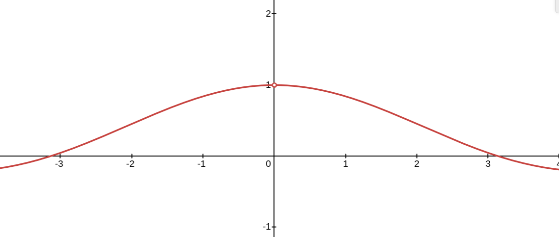
Suppose we wish to determine the slope of the tangent line (derivative) of \(f(x) = \sin x\) at \(x=0\text{.}\) We form the usual difference quotient: \(D(x)=\frac{\sin x - \sin
0}{x-0}=\frac{\sin x
}{x}\text{.}\)
From the graph, it might first appear that \(D(0) =1\) but we must be careful. \(D(0)\) doesn’t even exist! Somehow we must convey the idea that \(D(x)\) will approach \(1\) as \(x\) approaches \(0\text{,}\) even though the function \(D(x)=\frac{\sin x }{x}\) is not defined at \(0\text{.}\) Cauchy’s idea was that even if \(D(0)\) is meaningless it must be that \(\limit{x}{0}{D(x)}=1\) because we can make \(D(x)\) differ from \(1\) by as little as we wish by taking \(x\) sufficiently close to zero ([8], p. 158).
Karl Weierstrass made these ideas precise and provided us with our modern formulation of the limit in his lectures on analysis at the University of Berlin (1859-60).
We say \(\limit{x}{a}{f(x)} =L\) provided that for each \(\eps\gt0\text{,}\) there exists a \(\delta\gt0\) such that if \(0\lt \abs{x-a}\lt \delta\) then \(\abs{f(x)-L}\lt
\eps\text{.}\)
There are a couple of observations about Definition 10.1.3 that are worth making explicit:
Notice that Definition 10.1.3 is very similar to the definition of continuity at a point. This is because the two concepts are very closely related. In fact we can readily see that a function \(f\) is continuous at \(x=a\) if and only if the limit of \(f(x)\) as \(x\) approaches \(a\) is \(f(a)\text{.}\)
The statement of Definition 10.1.3 does not reflect the way we think or speak about limits at all. We speak of \(x\) getting close to, or approaching \(a\) which clearly indicates some sort of metaphorical motion. But the definition only references a single, unspecified and fixed parameter \(\eps{}\text{.}\) Once \(\eps \) is given if we need to find a value of \(\delta{}\) which guarantees that the inequality \(\abs{f(x)-L}\lt \eps \) holds as long as the inequality \(0\lt \abs{x-a}\lt \delta\) holds. In that case the limit exists and has the value \(L\text{.}\) There is no motion metaphorical or otherwise. We just have unchanging inequalities.
However, although \(\eps \) is fixed it is also unspecified. This means that once an appropriate \(\delta{}\) is found (usually in terms of \(\eps{}\)) then our inequalities will hold for every value of \(\eps{}\text{.}\) The upshot is that \(\eps \) represents every possible positive real number and \(\delta{}\) represent every corresponding response. There is no need for motion as a metaphor because all possibilities are handled at once.
This may seem unnecessarily complex to you and it certainly is complex. But it is also necessary because we want to use our mathematics to (among other things) interpret and explain the natural world. Using our intuition regarding motion (part of the natural world) to explain our mathematics would be reasoning in a circular fashion which is useless.
There are really only two differences between Definition 10.1.3 and Definition 8.1.7 and the differences are related. The first is that in the definition of a limit \(L\) plays the same role that \(f(a)\) played in the definition of continuity. This is because the function may not be defined at \(a\text{,}\) let alone have a value equal to \(L\text{.}\) In a sense the limiting value \(L\) is the value \(f\) would have if it was defined and continuous at \(a\text{.}\)
in the limit definition. You can see why this change is needed from the limit in Example 10.1.1. Since \(\frac{\sin
x}{x}\) is not defined at \(x=0\) we need to eliminate that possibility from consideration. This is the only purpose for this change.
Use Definition 8.1.7 and Definition 10.1.3 to prove that a function \(f(x)\) is continuous at \(x=a\) if and only if \(\limit{x}{a}{f(x)}=f(a)\text{.}\)
Consider the function \(\frac{x^2-1}{x-1}\text{,}\) where \(x\neq 1\text{,}\) which you probably recognize as the difference quotient used to compute the derivative of \(f(x)=x^2\) at \(x=1\text{,}\) so we strongly suspect that
Let \(\eps>0\text{.}\) We wish to find a \(\delta>0\) such that if \(0\lt \abs{x-1}\lt \delta\) then \(\abs{\frac{x^2-1}{x-1}-2}\lt \eps\text{.}\) With this in mind, we perform the following calculations
As in our previous work with sequences and continuity, notice that the scrapwork is not part of the formal proof (though it was necessary to determine an appropriate \(\delta)\text{.}\) Also, notice that \(0\lt \abs{x-1}\) was not really used except to ensure that \(x\neq 1\text{.}\)
Although it is rigorous Definition 10.1.3 is quite cumbersome to use. What we need to do is develop some tools we can use without having to refer directly to the definition. One such tool is Theorem 8.2.1 which allows us to show that a function is continuous (or discontinuous) at a point by examining certain sequences.
As we observed earlier, \(f(x)\) is continuous at \(x=a\) if and only if \(\limit{x}{a}{f(x)} = f(a)\text{.}\) On the other hand if \(f(x)\) is not continuous at \(x=a\text{,}\) but \(\limit{x}{a}{f(x)}=L \text{,}\) we can make it continuous by arbitrarily assigning \(f(a)=L\text{.}\) Combining this with Theorem 8.2.1 we have the following corollary:
\(\limit{x}{a}{\left(\frac{f(x)}{g(x)}\right)}=L/M\) provided \(M\ne0\) and \(g(x)\ne{}0\text{,}\) for \(x\) sufficiently close to a (but not equal to \(a\)).
Let \(\left(x_n\right)\) be a sequence such that \(x_n\ne a\) and \(\limit{n}{\infty}{x_n}=a\text{.}\) Since \(\limit{x}{a}{f(x)} = L\) and \(\limit{x}{a}{g(x)} = M\) we see that \(\limit{n}{\infty}{f(x_n)} = L\) and \(\limit{n}{\infty}{g(x_n)} = M\text{.}\) By Theorem 6.2.4 we have \(\limit{n}{\infty}{f(x_n)+g(x_n)}=L+M\text{.}\) Since \(\left(x_n\right)\) was an arbitrary sequence with \(x_n\ne a\) and \(\limit{n}{\infty}{x_n} = a\) we have
Suppose \(f(x)\le g(x) \le h(x)\text{,}\) for \(x\) sufficiently close to \(a\) (but not equal to \(a\)). If \(\limit{x}{a}{f(x)}=L=\limit{x}{a}{h(x)}\text{,}\) then \(\limit{x}{a}{g(x)}=L\) also.
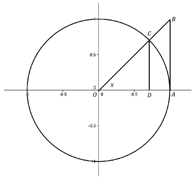
Returning to Example 10.1.1 we see that the Squeeze Theorem is just what we need. First notice that since \(D(x)=\frac{\sin x}{x}\) is an even function, we only need to focus on \(x\gt0\) in our inequalities. Consider the unit circle seen in Figure 10.1.15.
Use the fact that \(\cos x\) and \(\frac{\sin
x}{x}\) are both even functions to show that equation (10.1.1) is also true for \(-\frac{\pi}{2}\lt x\lt 0\)
Prove that if \(L\gt0\text{,}\) then there exists a \(\delta >0\text{,}\) such that if \(0\lt\left|x-a\right|\lt\delta \text{,}\) then \(f\left(x\right)>0\text{.}\)
Prove that if \(L\lt0\text{,}\) then there exists a \(\delta >0\text{,}\) such that if \(0\lt\left|x-a\right|\lt\delta
\text{,}\) then \(f\left(x\right)\lt0\text{.}\)
Notice that if \(\limit{x}{a}{f(x)}=L\text{,}\) then the contrapositive of part (a) says that if for each \(\delta >0\text{,}\) there is an \(x\) with \(0\lt\left|x-a\right|\lt\delta \) and \(f\left(x\right)\le
0\text{,}\) then \(L\le 0\text{.}\)
We say that a function \(f(x)\) has a property for \(x\) near \(a\text{,}\) if there exists a \({\delta }_0>0\) such that \(f(x)\) has that property for all \(x\) with \(0\lt\left|x-a\right|\lt{\delta
}_0\)
Section10.2The Definition of the Derivative and the Mean Value Theorem
As we mentioned in Section 3.1 Leibniz invented his calculus differentialis (differential calculus — literally “rules for (infinitely small) differences”) in the \(1600\)s.
In the late \(1700\)s Lagrange tried to provide a rigorous foundation for Calculus by discarding differential ratios like the expression \(\dfdx{y}{x} \) in favor of his own “prime notation” (\(f^\prime(x) \)). Thus it was Lagrange who established functions and limits, rather than the curves and infinitesimals favored by Leibniz and Newton, as fundamental.
When you took Calculus you spent at least an entire semester learning about the properties of the derivative and how to use them to explore the properties of functions so there is no need to repeat that effort here. Instead we will establish the underlying, rigorous, formal foundation for the derivative concept in terms of limits.
The derivative is defined at a point. If the derivative of \(f(x)\) is defined at every point in an interval \((a,b)\) then we say that \(f\) is differentiable on the interval \((a,b)\text{.}\)
Since it is defined as a limit, Corollary 10.1.8 applies. That is, \(f^\prime(x)\) exists if and only if \(\forall \text{ sequences } (h_n),\, h_n\ne
0\text{,}\) if \(\limit{n}{\infty}{h_n}=0\) then
Although it is an extraordinarily useful mathematical tool, it is not our intention to learn to use the derivative here. You did that in your Calculus course. Our purpose here is to define it rigorously (done) and to show that our formal definition does in fact recover the useful properties you came to know and love in your Calculus course.
Suppose \(f(c)\) is a maximum so that \(f\left(c\right)\ge
f(x)\) for all \(x\in (a,b)\text{.}\) Since \(f\) is differentiable at \(c\text{,}\) we have
It would be difficult to prove the MVT right now, so we will first state and prove Rolle’s Theorem, which can be seen as a special case of the MVT. The proof of the MVT will then follow easily.
Michel Rolle (1652–1719) first stated the following theorem in 1691. Given this date and the nature of the theorem it would be reasonable to suppose that Rolle was one of the early developers of Calculus but this is not so. In fact, Rolle was disdainful of both Newton and Leibniz’ versions of Calculus, once deriding them as a collection of “ingenious fallacies.” It is a bit ironic that his theorem is so fundamental to the modern development of the Calculus he ridiculed.
By the EVT, we know that \(f\) has a maximum \(M\text{,}\) and a minimum \(m\text{,}\) on \([a,b]\text{.}\) Suppose that both occur at the endpoints. This would say that \(m=M\) and \(f\) is constant on \([a,b]\text{.}\) What does this say about \(f^\prime\text{?}\)
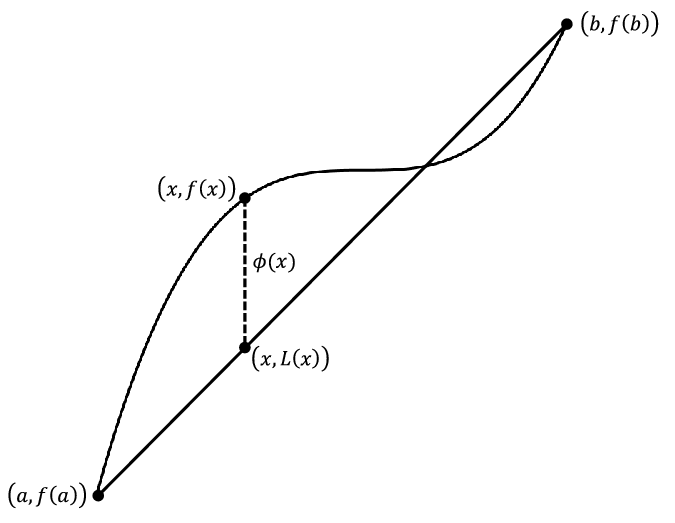
We can now prove the MVT as a corollary of Rolle’s Theorem. We only need to find the right function to apply Rolle’s Theorem to. The following figure shows a function, \(f(x)\text{,}\) cut by a secant line, \(L(x)\text{,}\) from \((a, f(a))\) to \((b,f(b))\text{.}\)
The Mean Value Theorem is extraordinarily useful. Almost all of the properties of the derivative that you used in Calculus follow more or less directly from it. For example the following is true.
Suppose \(c\) and \(d\) are as described in the corollary. Then by the Mean Value Theorem there is some number, say \(\alpha\in(c,d)\subseteq(a,b)\) such that
Suppose \(f\) is differentiable on some interval \((a,b)\text{,}\)\(f^\prime\) is continuous on \((a,b)\text{,}\) and that \(f^\prime(c)>0\) for some \(c\in (a,b)\text{.}\) Then there is an interval, \(I\subset (a,b)\text{,}\) containing \(c\) such that for every \(x, y\) in \(I\) where \(x\ge y\text{,}\)\(f(x)\ge f(y)\text{.}\)
Suppose that \(f\) is differentiable on some interval \((a,b)\text{,}\) and \(f^\prime \) is continuous on \((a,b)\text{.}\) If \(f^\prime(c)\lt 0\) for some \(c\in
(a,b)\) then there is an interval, \(I\subset (a,b)\text{,}\) containing \(c\) such that for every \(x, y\) in \(I\) where \(x\ge y\text{,}\)\(f(x)\le f(y)\text{.}\)
Suppose \(f(x)\) and \(g(x)\) are continuous on \([a,b]\) with \(f^\prime(x)=g^\prime(x)\) on \((a,b)\text{.}\) Show that \(f(x)=g(x)+C\) for some constant \(C\) on \([a,b]\text{.}\)
If you look back at our derivation of the Integral Form of the Remainder for Taylor Series (Theorem 4.1.12) you’ll see that the Fundamental Theorem of Calculus provided our anchoring step:
The Fundamental Theorem of Calculus was understood (in at least the limited context of polynomials) before Newton and Leibniz invented Calculus. They both provided derivations of it via their versions of Calculus, but again neither of them dubbed it “The Fundamental Theorem.” That name was an innovation of twentieth century Calculus textbooks. Both Newton and Leibniz considered it very natural and obvious that areas can be found by antidifferentiation.
Notice that equation (10.3.1) states that two differentials are equal. Thus it seems apparent that if we add (integrate) together all such differentials between \(x=a\) and \(x=b\) we have (again employing Leibniz’ notation)
Leibniz assumed that this is also true for an infinite sum of infinitesimals. This is probably the most intuitive possible understanding of the Fundamental Theorem of Calculus. In Leibniz’ notation it is
For Leibniz, this is all so natural and obvious that when he wrote about it in his 1693 paper Supplementum geometriae dimensoriae, seu generalissima omnium tetragonismorum effectio per motum: similiterque multiplex constructio lineae ex data tangentium conditione (More on geometric measurement, or most generally of all practicing of quadrilateralization through motion: likewise many ways to construct a curve from a given condition on its tangents) he called it a “supplementum” (supplement, or corollary) rather than something more imposing — like the Fundamental Theorem of Calculus.
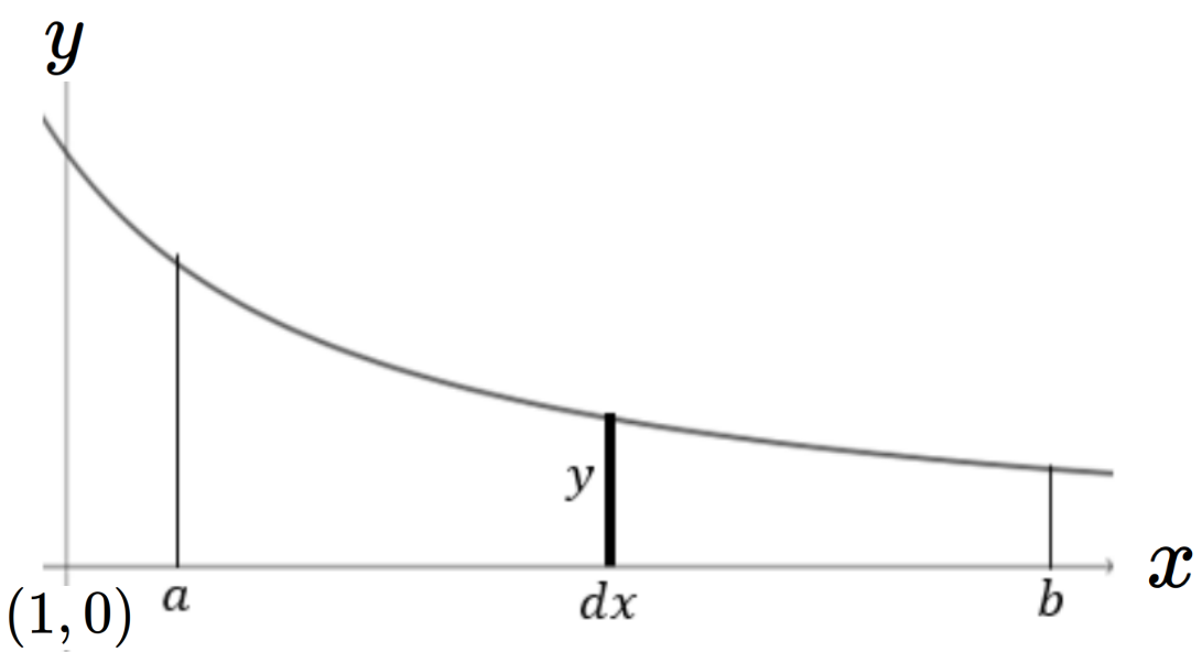
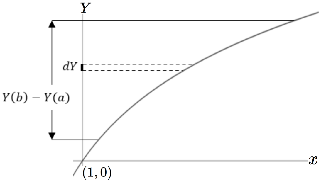
Leibniz rather famously favored very complex diagrams to illustrate his idea and he included one such diagram in his paper. We provide a simpler, more modern rendition below.
Figure10.3.1.A visual interpretation of the Fundamental Theorem of Calculus as it was understood by Leibniz. The relationship between the curves is that the function on the left, \(y=y(x)\text{,}\) is the derivative of the function on the right, \(Y=Y(x)\text{.}\)
In Figure 10.3.1 the area of the infinitely thin rectangle on the left is given by \(y\dx{x}\) and is numerically equal to the infinitely small length \(\dx{Y}\) on the right. Adding the areas on the left gives the area under the curve \(y(x)\) between \(a\) and \(b\text{.}\) The sum of the lengths on the right gives the length of the line segment, also between \(Y(a)\) and \(Y(b)\text{:}\)\(Y\left(b\right)-Y(a)\text{.}\)
Such an approach does not pass modern, or even \(19\)th century, standards of rigor. Even in the \(17\)th century it was known that there are logical problems with interpreting an integral in terms of infinitiesimals. But the infinitesimal approach was adequate to the needs of the time so a closer investigation into the nature of the integral was left until infinitesimals were no longer sufficient.
At this point we have all of the tools necessary for a rigorous proof of the Fundamental Theorem of Calculus. What we do not have is an adequate definition of the integral. We’ll need a definition that is independent of differentiation, but which recovers all of the properties of integration that you are already familiar with from your Calculus course, including the Fundamental Theorem of Calculus.
We’ll provide such a definition in Section 10.4 (the next section), but since we are already familiar with the properties we’ll need we will proceed with the proof of the Fundamental Theorem of Calculus now.
The following formulation and proof of the Fundamental Theorem of Calculus is from Cauchy’s 1823 publication Résumé des leçons donnés à l’ école royale polytechnique sur le calcul infinitesimal (Summary of the lessons given at the Royal Polytechnic School on infinitesimal calculus).
Equation (10.3.3) starts with the assumption that \(\dfdx{Y}{x}=y \text{.}\) It says that if we sum the differentials \(y\dx{x}\) from \(x=a\) to \(x=b\) then the sum collapses to the difference of the extremes: \(Y(b)-Y(a)\text{.}\)
On the other hand Theorem 10.3.3 starts with the assumption that \(\int_{t=a}^x f(t)\dx{t}\) is well defined, uses this to define the function \(I(x)\) ( which is simply \(Y(x)\) by another name), and then concludes where Leibniz began — with the statement that \(I^\prime
(x)=f(x)\text{,}\) (or \(\dfdx{Y}{x}=y\)). Our task in the next section will be to provide a definition that will support that conclusion.
In most Calculus texts equation (10.3.3) is called a definite integral, and the function defined in Theorem 10.3.3 is called an indefinite integral. The two of them are often referred to as parts \(1\) and \(2\) of the Fundamental Theorem of Calculus.
We will now proceed with the proof of Cauchy’s version of the Fundamental Theorem of Calculus, with the caveat that the proof is not complete until we have defined the function \(I(x)=\int_{t=a}^x f(t)\dx{t}\) and shown that under our definition it has the properties we expect from an integral. We will need some of these properties in the proof below.
We will prove differentiablity on \((a,b)\) first. From that continuity on \((a,b)\) follows immediately (why?). Continuity at the endpoints will be addressed separately.
We need to show that the limit in equation (10.3.4) is \(f(x)\text{.}\) Since \(f(t)\) was assumed to be continuous on \([a,b]\) it is also continuous on the closed interval with endpoints \(x\) and \(x+h\text{.}\) We know from the Extreme Value Theorem that there are points \(c\text{,}\) and \(C\text{,}\) in the same interval such that \(f(c)\) and \(f(C)\) are the global minimum and maximum of \(f\) on the closed interval with endpoints \(x\) and \(x+h\text{,}\) respectively.
Suppose \(f(x)\) is continuous on \([a,b]\) and \(I(x)\) is the antiderivative of \(f(x)\) from Theorem 10.3.3. Suppose further that \(F(x)\) is continuous on \([a,b]\) with \(F^\prime
(x)=f(x)\) on \((a,b)\text{.}\)
In a letter to Eratosthenes (circa 250 BC), Archimedes described what he called a mechanical method for finding areas and volumes. His method consisted of mentally dividing objects into infinitely thin slices and balancing these slices on an imaginary balance. Archimedes noted that while his method was not rigorous it was still quite useful. He said:
“. . . I thought it might be appropriate to write down for you a special method, by means of which you will be able to recognize certain mathematical questions with the aid of mechanics. I am convinced that this is no less useful than finding the proofs of these same theorems.”
“Some things, which first became clear to me by the mechanical method, were afterwards proved geometrically, because their investigation by that method does not furnish an actual demonstration. It is easier to supply the proof when we have previously acquired, by the method, some knowledge of the questions than it is to find it without any previous knowledge . . .”
Closer to our time Cavalieri, Torricelli, Kepler, Galileo, Roberval, and others explored a similar idea. They mentally cut geometric areas (and volumes) into infinitely thin slices. But rather than using an imaginary balance they compared them geometrically.
This division of objects into infinitely small pieces in order to analyze them is the essential idea underlying integration. As Archimedes observed it is questionable as a method of proof, but for practical applicatons this is still a useful way to think about problems.
It was always recognized that the notion of an infinitesimal was problematic as a logical foundation for Calculus but it was not until the beginning of the \(19\)th century that it became imperative to replace them (in large part due to the work of Fourier) with a more rigorous formulation.
Fourier’s work raises the question: How random can a function defined on an interval be and still be represented by a Fourier series? Since the coefficients are computed via integration, a closely related question is how random can a function be and still be integrable?
Since this text is intended as a one semester introduction to real analysis we will not be able to fully answer that question here. But we will give two equivalent rigorous definitions of the integral and then show that a continuous function on a closed interval is integrable. This will close the gap in our proof of the Fundamental Theorem of Calculus.
Subsection10.4.1Cauchy’s Definition of the Integral
One of the first mathematicians to provide a rigorous definition of a definite integral was Augustin Louis Cauchy in 1823. Cauchy used the limit idea to bridge the gap between finite sums of (finitely many) very small (but still finite) pieces and infinite sums of infinitesimals.
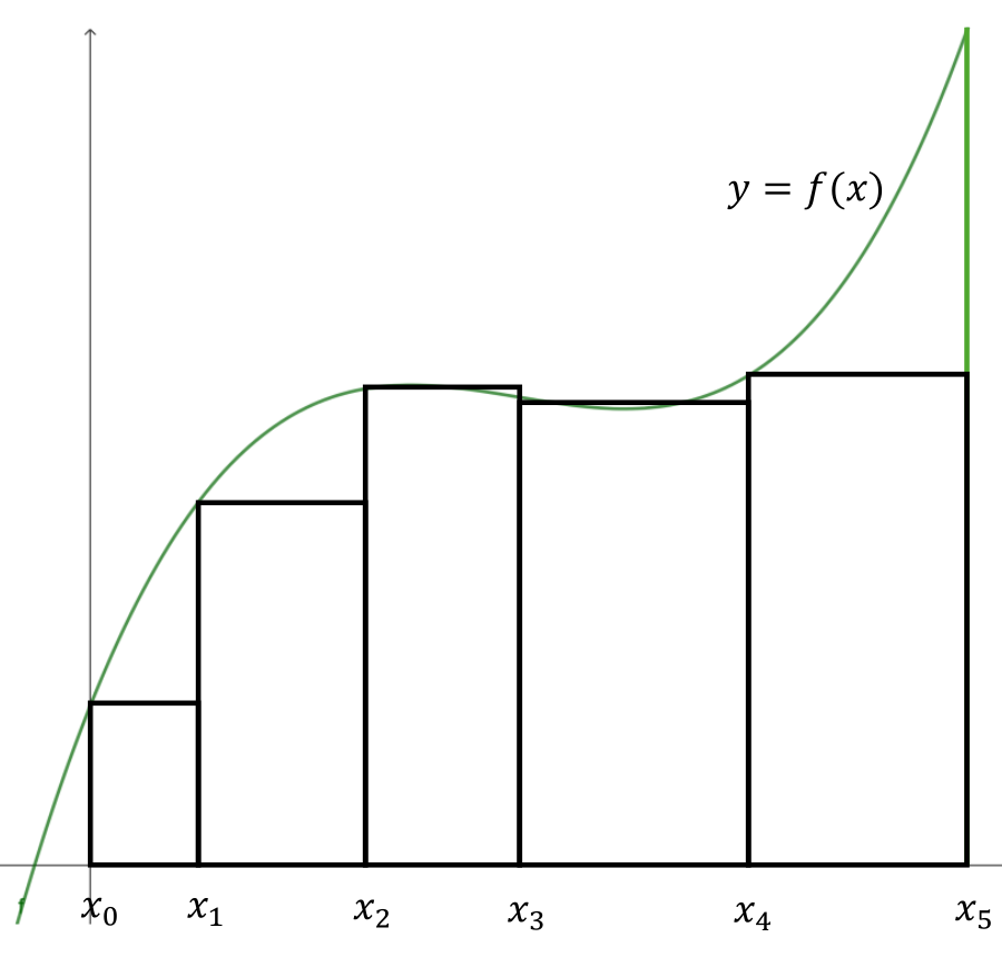
To approximate \(\int^b_{x=a}{f(x)\dx{x}}\text{,}\) Cauchy started by partitioning \(P\) of the interval\([a,b]\) into a finite number of subintervals. Basically, the partition \(P\) is a finite sequence of numbers
If \(f\left(x\right)\ge 0\) as in Figure 10.4.1 we see that we are approximating the area under the curve \(y=f(x)\) with the area of a finite sum of boxes whose bases are the subintervals \([x_k,x_{k+1}]\) and whose heights are obtained by evaluating \(f\) at some point in \([x_k,x_{k+1}]\text{.}\) In our figure we used the left endpoint \(x_k\) for convenience. Notice that the subintervals need not be the same length.
Diagrams like this are the source of the common misunderstanding that an integral computes area. In certain special cases it does, and it is often helpful to think of an integral as if it is an area but area is only one possible application of the integral. There are many others.
Cauchy said that a function \(f(x)\) defined on \([a,b]\) was integrable if there was a number \(I\) such that for all \(\eps >0\text{,}\) there is a \(\delta >0\) such that whenever the norm of the partition, \(\norm{P}\) is less than \(\delta{}\) the difference between \(I\) and the associated sum will be less than \(\eps{}\text{.}\) Symbolically this is
Using this definition Cauchy was then able to show that any continuous function is (Cauchy) integrable and was able to prove the Fundamental Theorem of Calculus as we indicated in the last section. More formally, Cauchy made the following definition.
Given a function \(f(x)\) defined on the interval \([a,b]\text{,}\) we say \(f\) is integrable on \([a,b]\) if and only if there is a number \(I\) such that for each \(\epsilon >0\text{,}\) there is a \(\delta >0\) such that for any partition \(P=\{x_0, x_1, \cdots, x_n\}\) of \([a,b]\) with \(\norm{P}\lt\delta \text{,}\) we have
The similarity between Definition 10.4.2 and the definition of a limit is hard to miss so sometimes the Riemann integral is defined via the limit symbol as
but in our (the authors’) opinions this notatation serves to hide the important ideas rather than elucidate them because the limit in equation (10.4.1) is very different from the ones we’ve encountered before.
In the past, when we had limits like \(\limitt{x}{2}{\frac{x^2-4}{x-2}}\) we only had to think about letting the single variable \(x\) get “close to” \(2\text{.}\) But the limit in equation (10.4.1) is far more complex. It asks us to simultaneously think about all possible partitions with the property that \(\norm{P}\lt\delta{}\text{,}\) and all possible choices of \(x_k^*\in \left[x_k,x_{k+1}\right]\text{,}\) in addition to what is happening when \(\norm{P} \rightarrow 0\text{.}\)
Because of these issues we will use an equivalent formulation of the definite integral. One which makes use of a concepts we’ve already familiar with: the least upper bound and greatest lower bound properties of the real number system.
Notice that neither the definition of the integral nor the definition of the derivative tells us how to compute the quantity in question. In the \(19\)th century the computational rules for both integrals and derivatives were as well understood as they are today. It was the logical support for these methods that was shaky. These definitions are about providing a rigorous foundation for these ideas, not about computing them.
In \(1875\)Jean Gaston Darboux (1842–1917) developed a different (but equivalent) definition of the Riemann integral which uses the least upper and greatest lower bounds we learned about in Chapter 9. We assume that \(f(x)\) is a bounded (not necessarily continuous) function on an interval \([a,b]\text{.}\)
As before, we will start with a partition \(P=\{x_0, x_1,x_2,
\dots , x_n\}\) of the interval \([a,b]\) where \(a=x_0\lt
x_1\lt \dots \lt x_{n-1}\lt x_n=b\text{.}\) Let \(m_k\) and \(M_k\) denote the infimum and supremum of \(f(x)\) on \([x_k,x_{k+1}]\text{,}\) respectively. Define the lower (Darboux) sum \(L(P)\) by
It is also intuitively clear that as the number of intervals gets larger, these bounds get closer to the actual integral (again, if it exists). If you don’t see this try drawing a few representative examples.
\(P^\prime \) is said to be a refinement of \(P\) if every point in \(P\) is also a point in \(P^\prime\text{.}\) That is, \(P\subset P^\prime \text{.}\)
Next observe that the set of lower sums over all partitions of \([a,b]\) is a non–empty set of real numbers which is bounded above. Therefore by Theorem 9.4.3 it has a least upper bound. We define the lower (Darboux) integral by
\begin{equation}
b
\underline{\int^b_{x=a}}{f(x)}\dx{x}=\sup_{P}
\left(L(P)\right)\tag{10.4.2}
\end{equation}
Similarly, the set of all upper sums is a non–empty set of real numbers which is bounded below and therefore has a greatest lower bound. We define the upper (Darboux) integral as the greatest lower bound of this set
Let \(P^\prime\) be a fixed partition of \([a,b]\text{.}\) By Problem 10.4.6, \(U(P^\prime)\) is an upper bound for the set of all lower sums. This says
Since Darboux’s integral is equivalent to the Riemann integral this definition does not guarantee that a given function will be Darboux (Riemann) integrable.
In honor of Dirichlet his function is often denoted \(D(x)\text{.}\) It is defined as follows:
\begin{equation}
D(x)=
\begin{cases}
0\amp \text{ if } x \text{ is irrational}\\
1\amp \text{ if } x \text{ is rational}
\text{.}\end{cases}\tag{10.4.4}
\end{equation}
As we mentioned earlier (but did not, and will not prove), Darboux’s definition of the integral is equivalent to the Riemann integral, in the sense that any function which is Riemann integrable is also Darboux integral and vice versa. This is similar to having both an analytic definition of continuity and a sequence–based definition of continuity. We can use whichever definition works better for the problem at hand.
For example, it is straightforward to derive the properties of definite integrals that you learned in Calculus using Cauchy’s formulation. But to show that a continuous function is integrable it is a little simpler to use Darboux’s formulation as we will see next.
Since \(f\) is continuous on \([a,b]\) it is continuous on each subinterval. Next define \(m_k\) and \(M_k\) to be the respective minimum and maximum of \(f(x)\) on the subinterval \([x_k, x_{k+1}]\text{.}\) If we choose a partition
We say alleged proof because there is a subtle problem. Because \(f(x)\) is continuous on \([a,b]\) it is continuous at each point \(x\in [a,b]\text{.}\) This says that for each \(x\text{,}\) there is a \({\delta }_x\gt 0\text{,}\) such that if \(\abs{x-y}\lt\delta_x\) then \(\left|f\left(x\right)-f\left(y\right)\right|\lt\frac{\epsilon
}{b-a}\text{.}\) But if you look at our sketch of the alleged proof you see that we need a single \(\delta >0\) which works uniformly for all such \(x, y\in [a,b]\text{.}\) This leads to the following definition.
Suppose \(S\subset \RR\text{.}\) We say that \(f(x)\) is uniformly continuous on \(S\) provided that for all \(\eps
>0\text{,}\) there is a \(\delta >0\) such that \(\left|f\left(x\right)-f\left(y\right)\right|\lt \eps \) for all \(x, y\in S\) with \(\left|x-y\right|\lt \delta \text{.}\)
This is called uniform continuity because a single value of \(\delta \) works uniformly for all \(x,y\in S\text{,}\) whereas in regular continuity, \(\delta \) may depend on the value of \(x\text{.}\) It is clear that any function which is uniformly continuous on a set \(S\) is continuous on \(S\text{,}\) but the converse is not always true. That is, uniform continuity is a stronger property than continuity.
Our “alleged proof” of Theorem 10.4.11 is in fact a valid proof that a uniformly continuous function is (Darboux) integrable. But as Problem 10.4.13 points out, a continuous function need not be uniformly continuous. The hypothesis of Theorem 10.4.11 requires that the function be defined on a closed bounded interval, so the difficulty in Problem 10.4.13 is that the interval \([0,\infty)\) while closed, is unbounded. The following lemma closes the gap.
We will do a proof by contradiction. Suppose \(f(x)\) is not uniformly continuous on \([a,b]\text{.}\) Then there is an \(\eps
>0\) such that for any \(\delta >0\text{,}\) there are \(x,y\) with \(\left|x-y\right|\lt \delta \) , but \(\left|f\left(x\right)-f\left(y\right)\right|\ge \eps \text{.}\) If we let \(\delta =\frac{1}{n}, n\in \mathbb{N}\text{,}\) then we can create two sequences \(\left(x_n\right), (y_n)\) with \(\left|x_n-y_n\right|\lt \frac{1}{n}\text{,}\) but \(\left|f\left(x_n\right)-f\left(y_n\right)\right|\ge \eps .\) By the Bolzano–Weierstrass Theorem, there is a \(c\in [a,b]\) and a subsequence \((x_{n_k})\) with \(\limit{k}{\infty }{ x_{n_k} }=c\text{.}\) Given how \((y_n)\) was constructed, \(\limit{k}{\infty }{ y_{n_k} }=c\text{.}\) Since \(f(x)\) is continuous at \(c\text{,}\) you should be able to get a contradiction out of this.
The evolution of the modern definition of a function is parallel to, and intertwined with, the definition of the definite integral. Issues of integrability were not prevalent in 18th century because for most of that time the words integral and antiderivative were synonymous. Thus the only integrable functions were the ones that were derivatives of some other function. But in the 19th century, and especially after Fourier, we needed to integrate functions that were not clearly derivatives of something else. As a result the need for a precise definition of function became more and more pressing as the years went by. For example, here is the definition of a function from Euler’s Introductio in Analysin Infinitorum (1748).
“A function of a variable quantity is an analytic expression composed in any way whatsoever of the variable quantity and numbers or constant quantities.”
This is the “function as input/output machine” metaphor that you’ve probably used all of your life so far: A number goes in, gears turn or electronic circuits are activated and a new number is generatied as output from those actions. The advent of Fourier series ushered in a need for a much more general definition. Here is Fourier’s definition from his Théorie analytique de la Chaleur (1822).
“In general, the function \(f(x)\) represents a succession of values or ordinates each of which is arbitrary. An infinity of values being given of the abscissa \(x\text{,}\) there are an equal number of ordinates\(f(x)\text{.}\) All have actual numerical values, either positive or negative or nul. We do not suppose these ordinates to be subject to a common law; they succeed each other in any manner whatever, and each of them is given as it were a single quantity.”
This is closer to our modern approach. In the modern definition for each \(x\) in the domain, there is a unique \(f(x)\) assigned to it. It is different from Euler’s definition in that no formula, and no metaphorical machine is needed to generate an output. A function can be defined by simply giving a list of ordered pairs. No particular rule is needed.