The brilliant Cerebron, . . . discovered three distinct kinds of dragon: the mythical, the chimerical, and the purely hypothetical. They were all, one might say, nonexistent, but each non-existed in an entirely different way.
In Subsection 9.5.4 we saw that those points where the derivative doesn’t exist are possible optimal points but we didn’t pursue this any further at the time. However we now need to re-examine the non-existence of derivatives.
We also observed in Subsection 9.5.4 that derivatives fail to exist at points where the Principle of Local Linearity 5.2.5 does not hold. This is true, but the only way we currently have to determine if the Principle of Local Linearity holds is to look at a graph. While graphs are useful, we have learned that we should not put all of our faith in conclusions drawn from graphs.
On the other hand, by Definition 13.2.3 the derivative of a function is given by a limit, and from our work in Chapter 12 we know that not all limits exist. For example, if we try to compute the value of \(f^\prime(2)\) for some function and we find that \(\tlimit{h}{0}{\frac{f(2+h)-f(2)}{h}}\) is meaningless then \(f\) is not differentiable at \(x=2\text{.}\) In other words, \(f^\prime(2)\) does not exist.
So, the limit definition gives us a computational tool we can use to decide the question of differentiability which, as we saw in Chapter 9.5, is crucial to finding possible optimal transition points of a function.
In our comments following Example 9.5.15 we listed several functions which are not differentiable at \(x=0\text{.}\) Of these, the Absolute Value function, \(f(x)=\abs{x}\text{,}\) is probably the simplest to work with, so we will start there.
The Absolute Value function is usually introduced with some vague statement like, “The absolute value of a number is just the positive version of the number,”
Or sometimes an appeal is made to the intutive notion of distance, as “\(\abs{x-a}\) gives the length of the line segment between \(x\) and \(a\text{.}\)”
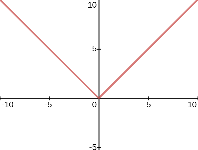
The graph of the Absolute Value function is given in Figure 16.1.3 below. Notice that \(f(x)=\abs{x}\) is defined at \(x=0\) since \(\abs{0}=0\text{,}\) but as we indicated in Subsection 9.5.4 the Principle of Local Linearity does not hold at \(x=0\) so we suspect that the Absolute Value function is not differentiable at \(x=0\text{.}\)
But we now have the ability to confirm our suspicion analytically so let’s take a look at this using the limit definition of the derivative. The derivative of \(\abs{x}\) at \(x\) will be the value of the limit \(\tlimit{h}{0}{\frac{\abs{x+h}-\abs{x}}{h}}\) so the derivative of \(\abs{x}\) at \(x=0\) will be:
OK, but what is this limit? Don’t jump to conclusions. Think about this carefully for a few minutes. What do you think \(\tlimit{h}{0}{\frac{\abs{h}}{h}}\) is equal to?
First suppose that \(h\) is approaching zero from the positive side. Recall that in Section 12.3 we invented the notation “\(\rlimit{h}{0}{} \)” for exactly this situation. In this case \(h\) is positive so \(\abs{h}=h\) and
But since \(\frac{\abs{h}}{h}\) can’t be close to \(1\) and close to \(-1\) simultaneously we can not find a value for \(\tlimit{h}{0}{\frac{\abs{0+h}-\abs{0}}{h}}\) which is correct for both positive and negative values of \(h\text{.}\) In other words this limit does not exist.
According to Definition 9.5.18, since \(\dfdxat{(\abs{x})}{x}{0}\) does not exist, the value \(x=0\) is a possible transition point for the Absolute Value function. So there might be a local extremum of \(f(x)=\abs{x}\) at \(x=0\text{.}\) Is there?
The Absolute Value function is not differentiable at \(x=0\) but it is differentiable at every other value of \(x\text{.}\) Let \(f(x)=\abs{x}\) and use Definition 13.2.3 to show that:
From the discussion in The Absolute Value Function we know that \(f(x)=\abs{x}=\sqrt{x^2}\text{.}\) Use the differentiation rules you learned in Part 1 of this text to show that if \(x\neq0\text{,}\) then \(f^\prime(x) = \frac{x}{\abs{x}}.\) How does this compare with your calculations part (a)
A slightly less intuitive example is the function \(f(x)=\frac{x}{x}\text{.}\) It is tempting to claim that this is really just \(f(x)=1\) since “anything divided by itself is one” but that claim is not true. As we saw in Dividing By Zero division by zero is undefined, regardless of the numerator. So the expression \(\frac00\) is undefined, and therefore the function \(f(x)=\frac{x}{x}\) is not defined at \(x=0\text{.}\) It is also tempting to try to invoke L’Hôpital’s Rule, since it is true that
But this only says that the limit of \(f(x)\) is equal to one, not that \(f(x)\) itself is equal to one, at \(x=0\text{.}\) As we’ve seen the statement \(\limit{x}{0}{\frac{x}{x}} = \limit{x}{0}{1}\) explicitly excludes the point \(x=0\) from consideration. This is why when we discussed indeterminate forms in Section 12.4 we were very careful to write \(\frac{\approach{0}}{\approach{0}}\) instead of \(\frac00\text{.}\) We needed to emphasize that we specifically do not allow the denominator to be equal to zero.
It is pretty clear that \(f^\prime(0)\) is undefined, since \(f(0)\) is undefined. We can’t have a derivative where we don’t have a point. But this is the kind of vague reasoning we are trying to avoid. Part (a) of this exercise shows unequivocally that the limit which defines \(f^\prime(0)\) is undefined.
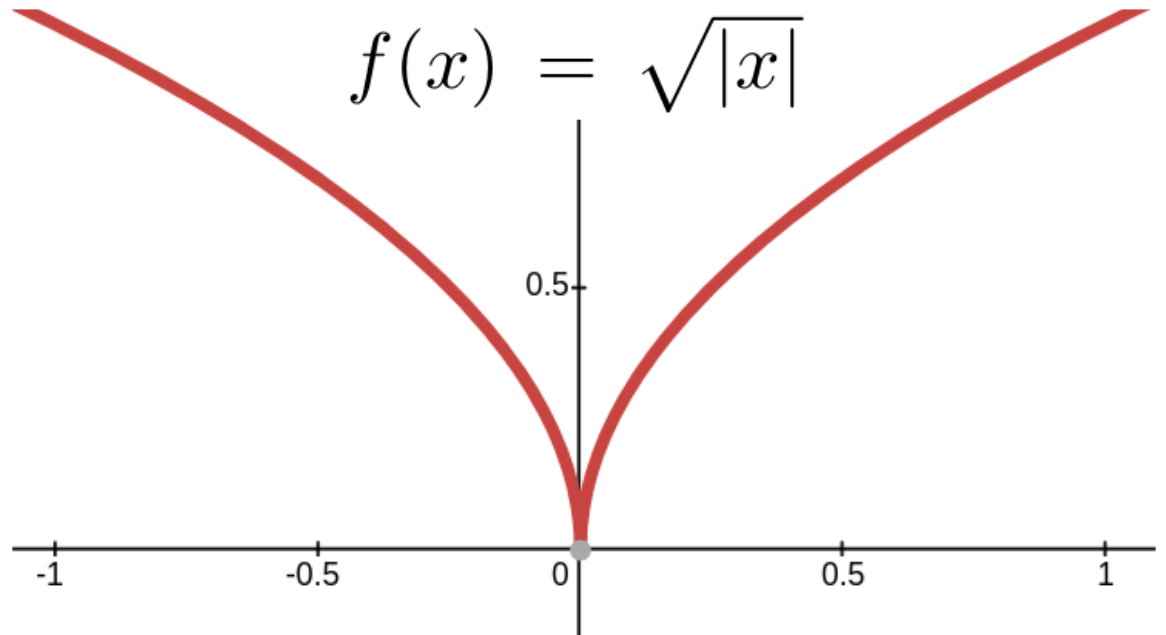
It is intuitively clear that derivative of the function \(f(x)=\sqrt{\abs{x}}\) (above) is not defined at \(x=0\text{.}\) We will confirm our intuition using Definition 13.2.3.
That is, we’ll try to compute the derivative of \(f(x)\) at \(x=0\) using Definition 13.2.3 and see what goes wrong. The existence of the derivative of \(f(x)\) at \(x=0\) is equivalent to the existence of the limit \(\tlimit{h}{0}{\frac{f(0+h)-f(0)}{h}}\text{,}\) so we will try to compute this limit and see what happens.
Problem 16.1.9 shows, \(\frac{\sqrt{\abs{h}}}{h}\) increases without bound as \(h\) approaches zero from the right, and decreases without bound as \(h\) approaches zero from the left. Since neither of these limits even exists it follows that \(\tlimit{h}{0}{\frac{\sqrt{\abs{h}}}{h}}\) also does not exist, and therefore \(f^\prime(0)\) is not defined.
Notice that it is not defined at \(x=0\text{.}\) We call \(H(x)\) the Heaviside function in honor of Oliver Heaviside (1850–1925). Simple as it is, Heaviside’s function is a fundamental tool in signal processing, control theory, and the solution of differential equations.
We first introduced one–sided limits in Section 12.3. At the time our concern was to locate vertical asymptotes so we only looked at limits that were equal to either positive or negative infinity. We see now that these limits can take any value and that they are more fundamental than they first appeared to be. We are still not quite ready for a formal definition but Definition 16.1.12 earlier we will do so now.
Because \(f(x)\) can’t simultaneously approach two different numbers, if the left– and right–hando limits both exist but do not agree then \(\limit{x}{a}{f(x)}\) doesn’t exist. This fact will be a useful tool for us later so we state it as a theorem.
Theorem 16.1.13 requires proof but we do not have the tools to prove it here. The appropriate tools will be developed in Chapter 17. Proving this fact is the last problem in this textbook.