Section12.4Indeterminate Forms and L’Hôpital’s Rule
Subsection12.4.1L’Hôpital’s Rule
Based on our experience so far it is tempting to conclude that we can locate vertical asymptotes by simply setting the denominator equal to zero and solving. But this is a naive conclusion as we will see next.
Consider \(y=\frac{x-2}{x^2-4}\text{.}\) Setting the denominator equal to zero yields \(x=-2\) and \(x=2\text{,}\) but only one of these is a vertical asymptote. Do you see which one?
Let’s take a careful look at this example. By Definition 12.3.1 we will have a vertical asymptote when either one-sided limit of a function increases or decreases without bound, so we must evaluate each one-sided limit.
We were careful to use one-sided limits to find the vertical asymptote at \(x= -2\) because this is what Definition 12.3.1 calls for. Strictly speaking we only needed one of them, but since these limits were not equal we evaluated them both.
Observe that this limit has the form \(\limit{x}{2}{\frac{x-2}{x^2-4}}=\frac{\approach{0}}{\approach{0}}\text{.}\) A limit of this form is another indeterminate Form like \(\approach{\infty -\infty }\text{.}\)
Example 12.4.1 demonstrates that a function which does not exist at a point is a more general concept than a function with a vertical asymptote at a point.
Notice that \(g(x)=\frac{x-2}{x^2-4}\) is undefined at both \(x=2\) and \(x=-2\text{,}\) but it only has an asymptote at \(x=-2\text{.}\) It also displays something subtle about limits. One would be tempted to say that
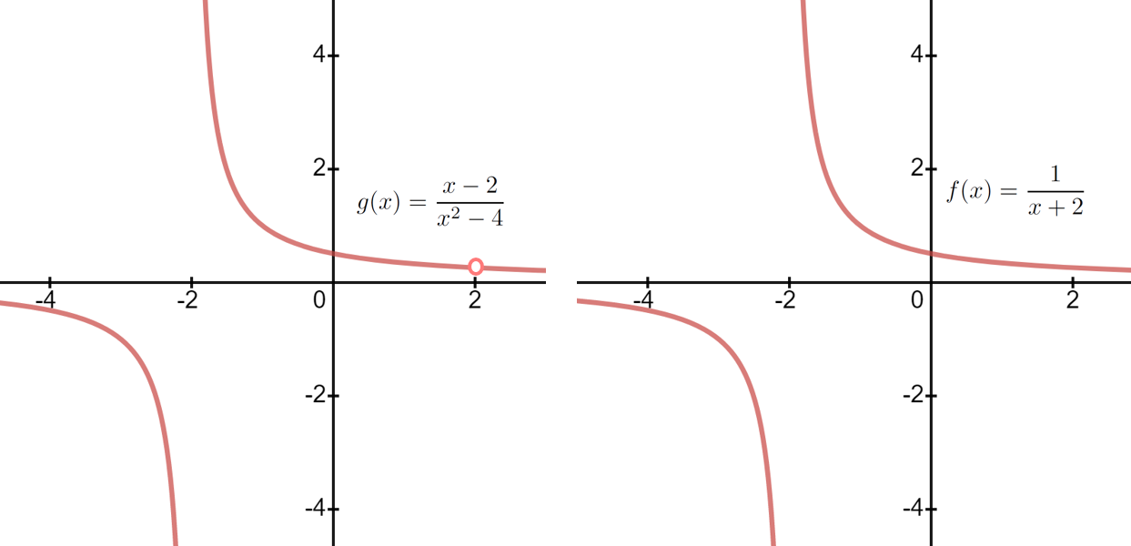
and this is true when \(x\neq2\text{.}\) However, if we graph the two functions, \(g(x)=\frac{x-2}{x^2-4}\) and \(f(x)=\frac{1}{x+2}\) we see that there is a small difference between them:
Do you see the difference? The value of \(g(2)\) is not defined because \(g(2)=\frac{2-2}{4-4}\) and we get a zero denominator. But no such difficulty occurs with \(f\) because \(f(2) = \frac{1}{2+2}=\frac14\text{.}\)
So, when \(x\neq2\text{,}\)\(g(x)\) and \(f(x)\) are the exactly the same. But they disagree when \(x=2\text{.}\) More precisely \(x=2\) is not in the domain of \(g(x)\) but it is in the domain of \(f(x)\text{.}\) Since the domains differ they must be different functions and it is incorrect to write \(\frac{x-2}{x^2-4}=\frac{1}{x+2}\) even though it is true for all but one value of \(x\text{.}\)
In that problem you showed that the fluents, \(x(t) =
\frac{3t}{1+t^3}\) and \(y(t)=\frac{3t^2}{1+t^3}\) satisfy the equation of the Folium:
\begin{equation*}
x^3+y^3=3xy
\end{equation*}
and that \(t=0\) is the only value of \(t\) where \(\left(x(t), y(t)
\right)=(0,0)\text{.}\) How then, can it be that the Folium crosses itself at the origin?
In Problem 5.9.3 you determined that \(y\ge0\) when \(t\gt-1\text{.}\) Determine the values of \(t\) for which \(x\ge0\) and the which \(x\lt0\text{.}\)
Compute \(\dfdx{y}{x} = \frac{\dot{y}}{\dot{x}}\) in terms of \(t\) and compute \(\limit{t}{\pm\infty}{\frac{\dot{y}}{\dot{x}}}\text{.}\) Is this consistent with what you see on the graph?
Show that for \(t\neq0\text{,}\)\(t=\frac{y}{x}\) so that geometrically, \(t\) represents the slope of the line joining the origin to the point \((x,y)\) on the graph of the Folium. Is this consistent with what you obtained in part a? Explain.
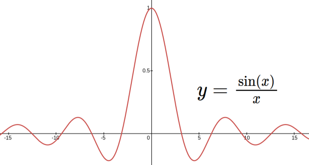
We found earlier that \(\tlimit{x}{\infty}{\frac{\sin(x)}{x}}=0\text{,}\) so the function \(y=\frac{\sin(x)}{x}\) must have a horizontal asymptote at \(y=0\text{.}\) Clearly \(y=\frac{\sin(x)}{x}\) is undefined at \(x=0\text{.}\) Does its graph have a vertical asymptote at \(x=0\text{?}\) Take your best guess.
To answer this question we need to evaluate the limit \(\tlimit{x}{0}{\frac{\sin(x)}{x}}\text{.}\) But how can we do that? If we try the obvious ploy of just “plugging in” zero for \(x\) we get the indeterminate form \(\frac{(\rightarrow0)}{(\rightarrow0)}\text{,}\) and we know we need to proceed cautiously with an indeterminate form.
From the graph of \(\frac{\sin(x) }{x}\) (in the sketch below) it would appear that \(\frac{\sin(x)}{x}\rightarrow1\) as \(x\rightarrow0\text{.}\) This is correct, but we’ve learned to be wary of relying on graphs. It would be best to evaluate the limit by another technique if possible.
It is hard to see what it would be. There isn’t much algebra we can do here. If there were other trigonometric functions involved we might be able to employ some trigonometric identity in the numerator, but there just isn’t much we can do with \(\sin(x)\text{.}\) This problem poses a bit more of a challenge than the indeterminate forms we have dealt with so far. We need a new idea.
Since the \(\sin(x)\) isn’t helping maybe we can replace it with something simpler. Seriously. Give some thought to what might be a valid replacement before reading on. Remember that we’re really only interested in values of \(x\) that are very close (infinitely close?) to zero.
The Principle of Local Linearity says that the graph of a function and its tangent line are locally indistinguishable. Since we’re only interested in values of \(x\) near zero — locally around zero — let’s try replacing \(\sin(x)\) with its tangent line.
also has the indeterminate form \(\frac{(\rightarrow0)}{(\rightarrow0)}\) so we’ll need the tangent lines of the numerator and denominator at \(x=0\) again.
Graph the equation \(y=\frac{\tan(3x)}{\sin(2x)}\) and zoom in on the portion of the graph near \(x=0\text{.}\) Does it look like we’ve found the correct limit?
In all of our examples where the indeterminate form was a fraction, replacing the numerator and denominator with their respective tangent lines seems to have worked. The idea seems promising so let’s look at it in a more general context. If \(f(x)\) and \(g(x)\) are differentiable functions such that \(f(a)=g(a)=0\) then \(\limit{x}{a}{\frac{f(x)}{g(x)}}\) is an indeterminate form.
(We’ll need to assume that \(g^\prime(a)\neq0\text{.}\) Do you see why?) This is consistent with all of our examples above so it appears that the Principle of Local Linearity has led us in the right direction. All of the evidence we’ve gathered so far suggests rather strongly that when we are faced with the indeterminate form \(\frac{(\rightarrow0)}{(\rightarrow0)}\) simply replacing the numerator and denominator with their tangent lines will work.
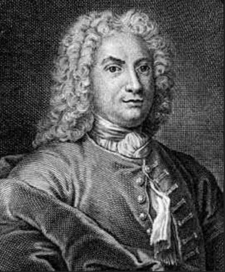
This idea is due to the Swiss mathematician Johann Bernoulli (1667–1748). Johann and his brother Jacob Bernoulli (1665–1795) were taught Calculus by Leibniz himself, but soon showed themselves to be his equal, or nearly so.
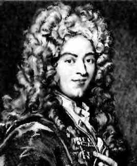
As a mathematician L’Hôpital was not in the same league as Leibniz, Newton, or the Bernoullis — few are — but he was a very competent mathematician and his work helped to disseminate the ideas of Calculus just as Maria Gaëtana Agnesi’s text would do in the following century.
Now look back at the examples in this section and notice the following fact: In each case when the limit was finally evaluated it turned out to be the slope of the line tangent to the graph of the numerator divided by the slope of the line tangent to the graph of the denominator. But the slope of the line tangent to \(f(x)\) at \(x=a\) is simply \(\eval{\dfdx{y}{x} }{x}{a} = f^\prime(a)
\text{.}\)
In light of equation (12.5) it appears that we don’t need to go to the trouble of finding the tangent lines. We can evaluate these indeterminate forms as follows:
Because L’Hôpital’s Rule applies directly to the indeterminate form \(\frac{(\rightarrow0)}{(\rightarrow0)}\) we will refer to this as a L’Hôpital Indeterminate. Not all indeterminate forms are L’Hôpital Indeterminates.
We want to emphasize very strongly that L’Hôpital’s Rule requires a L’Hôpital indeterminate. If we don’t have a L’Hôpital indeterminate we can not use L’Hôpital’s Rule. If you try to use L’Hôpital’s Rule when it does not apply, you will probably not get the correct answer. The difficulty here is that nothing in the computations will alert you that anything has gone wrong. You have to be watchful for this potential pitfall.
For example, if we mistakenly try to use L’Hôpital’s Rule, on \(\limit{x}{1}{\frac{x+1}{x+2}}\) we will obtain \(\limit{x}{1}{\frac{1}{1}}=1\text{,}\) but this is obviously incorrect.
Theorem 12.4.15 is useful but it is much too limited, so to speak. For example, it does not help us with this limit: \(\tlimit{x}{0}{\frac{\cos(3x)-1}{\cos(5x)-1}}\text{.}\) Even though it is a L’Hôpital indeterminate, when we apply Theorem 12.4.15 we have
Our derivation of Theorem 12.4.23 is not entirely rigorous. We will not be providing a fully rigorous derivation of L’Hôpital’s Rule because doing so is both difficult to produce and to understand. There are deep foundational issues involved and investigating these would take us too far from our primary purpose, gaining proficiency with its use. Returning to our example and using Theorem 12.4.23 this time we have
Use Theorem 12.4.23 to compute each of the following limits. If this limit given is not a L’Hôpital Indeterminate rearrange it algebraically, without changing its value, until it is a L’Hôpital Indeterminate.
Subsection12.4.2L’Hôpital’s Rule and Horizontal Asymptotes
Our discovery of L’Hôpital’s Rule grew from our investigation of vertical asymptotes. Is there any way that we can extend L’Hôpital’s Rule to help us with horizontal asymptotes? For example, consider
This limit is indeterminate of the form \(\frac{(\rightarrow0)}{(\rightarrow0)}\text{,}\) so it seems like L’Hôpital’s Rule would apply. But both versions of L’Hôpital’s Rule (so far) require that \(x\rightarrow
a,\) where \(a\) is a real number. And of course, infinity still insists on not being a number, real or otherwise. If we want to use L’Hôpital’s Rule we’ll have to find a way to modify this limit so that L’Hôpital’s Rule does apply.
Far more important than the answer in this example is the realization that we can use the same trick to extend L’Hôpital’s Rule to the case where \(x\) approaches both \(\infty,\) and \(-\infty.\)
To see this in the general situation suppose that \(\limit{x}{\infty}{f(x)}=0\) and \(\limit{x}{\infty}{g(x)}=0.\) If we make the substitution \(z=\frac{1}{x}\) then as \(x\rightarrow\infty\) we have one-sided limits as \(z\) approaches zero from the right side. Now we can use L’Hôpital’s Rule with \(z\) as the variable:
Although we have not discussed it here, L’Hôpital’s Rule also applies directly to the indeterminate form \(\frac{\approach{\pm\infty}}{\approach{\pm\infty}}\text{,}\) as well as \(\frac{\approach{0}}{\approach{0}}\text{.}\) So we will also call these L’Hôpital Indeterminates.
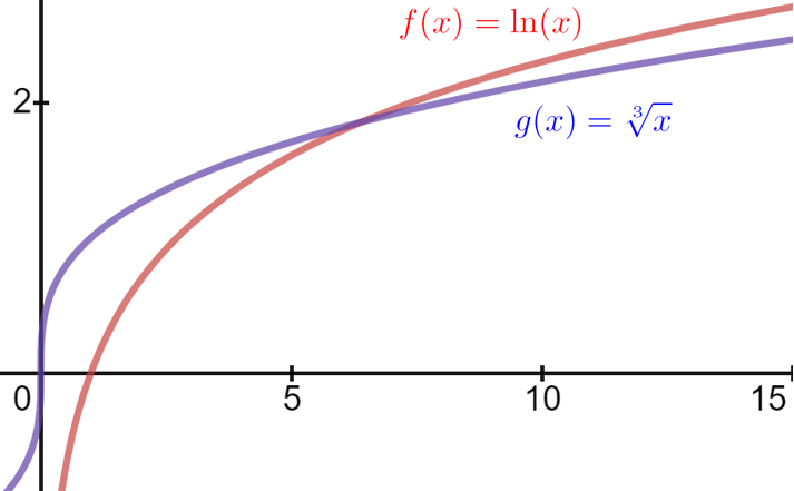
As \(x\rightarrow\infty\) both \(f(x)=\ln(x)\) and \(g(x)=\sqrt[3]{x}\) increase without bound, but which one increases faster? Take a quick look at the graphs below.
As \(x\rightarrow\infty\) both graphs are flattening out, but it would appear that the natural logarithm function is outgrowing the cube root function. Is it? We can answer this question by looking at the limit,
If the limit is \(\infty\) then \(f(x)=\ln(x)\) is growing faster. If it is zero then \(g(x) = \sqrt[3]{x}\) is increasing faster than \(f(x)=\ln(x).\) (Do you see why?)
Colloquially, the phrase “exponential growth” just means that something is growing very fast, but it has a more precise meaning in mathematics. It means the growth rate is described by an exponential function. For example neither \(f(x)=x^2\) nor \(f(x)=x^{200}\) grows exponentially. They are both said to grow “polynomially”. But \(f(x) = e^x\text{,}\)\(f(x)=2^x\text{,}\) and even \(f(x)=1.0001^x\) all do grow exponentially The next problem explores how “exponential growth” compares “polynomial growth.”
Suppose that \(P(x)\) any polynomial and show that \(\limit{x}{\infty}{\frac{P(x)}{e^x}}=0\text{.}\) Do you see that this means that the natural exponential grows faster than any polynomial?
\begin{equation*}
\limit{x}{\infty}{ \left[ x \tan\left(\frac1x\right)
\right]}.
\end{equation*}
If we want to evaluate this limit (we do) we seem to have few options. This is not a L’Hôpital Indeterminate, nor is it obvious what the limit might be. Simply letting \(x\rightarrow\infty\) we see that \(x\rightarrow\infty\) and \(\tan\left(\frac1x\right)\rightarrow0\) so our limit has the Indeterminate form \(\approach{\infty}\cdot\approach{0}\text{.}\)
There is a real temptation to say that this must be zero since anything multiplied by zero is zero. But is it? Remember that the purpose of the arrow notation, \((\rightarrow0)\text{,}\) is to remind us that the expression \(\tan\left(\frac{1}{x}\right)\) is never actually equal to zero. It merely approaches zero. At the same time \(x\) is increasing without bound (\(x\rightarrow\infty\)) so it seems that the value of the limit might depend on the relative speeds with which \(x\rightarrow\infty\) and \(\tan\left(\frac{1}{x}\right)\rightarrow0\text{.}\)
But this reasoning feels very uncertain doesn’t it? And, in any case, nothing we’ve said will help us evaluate the limit. We’ll have to find a way to re–express this limit as a L’Hôpital Indeterminate so that L’Hôpital’s Rule does apply. In the meantime, take your best guess as to the value of this limit and write it down for later reference. Suppose we rewrite this limit as
\begin{equation*}
\limit{x}{\infty}{ \left[ x \tan\left(\frac1x\right) \right]} =
\limit{x}{\infty}{\frac{\tan\left(\frac1x\right)}{\frac1x}}.
\end{equation*}
This is a little scary to look at so we’ll make it easier on our eyes with the substitution \(z=\frac1x\text{.}\) As \(x\rightarrow\infty\) we see that \(z\gt0\) and \(z\rightarrow0\text{.}\) Since \(\tan(0)=0\) our limit is now \(\rlimit{z}{0}{\frac{\tan\left(z\right)}{z}}\) which is the L’Hôpital Indeterminate \(\frac{(\rightarrow0)}{(\rightarrow0)}\text{.}\) Thus by Theorem 12.4.25 we have
Notice that the trick we used was a simple substitution much like the ones we have used in the past to make things “easier on the eyes.” The difference here is that we’re not making anything “easier on the eyes.” If anything we’re making things harder to look at since re–writing \(x\) as \(\frac{1}{\frac1x}\) certainly doesn’t seem like it’s going to help much. Until we try it. Always try your ideas out no matter how crazy they seem to be. Only after you try an idea can you tell if it will work or not.
Recall that in Section 8.2 where we defined the effective yield of an investment which is compounded continuously. We were led to examine the expression \(\left(1+\frac{1}{m}\right)^m\) for very large values of \(m\text{.}\)
As a result of that investigation we accumulated considerable numerical evidence that in one year an investment of \(1\) growing at a nominal rate of \(5\%\text{,}\) compounded continuously would grow to \(e^{0.05}\approx 1.0513\text{,}\) but we were unable to do more than gather evidence. It was pretty convincing evidence but it was not proof since we didn’t yet have the mathematical technique necessary to evaluate the expression \(\left(1+\frac{1}{m}\right)^m\) as \(m\rightarrow\infty\text{.}\) Now we do.
It is tempting to reason as follows. We see that \(1+\frac{1}{m}\rightarrow1\) as \(m\rightarrow\infty\text{.}\) That is, we have the indeterminate form \(\approach{1}^{\approach{\infty}}\) and since one raised to any power is equal to one this limit must equal \(1\text{,}\) right? Surely you know better than to jump to that conclusion by now. Not only does all of the evidence of this chapter warn you that limits are more subtle than that, but in our investigations in Section 8.2 we saw overwhelming evidence that this limit is not equal to one.
The source of our difficulty here is that the variable \(m\) is in the exponent where we can’t get at it. We’d like to find a way to bring it out of the exponent. The natural logarithm seems perfect for this task since it has the property that \(\ln\left(a^b\right)=b\ln(a)\text{.}\)
The limit on the right is an indeterminate form but unfortunately it is not a L’Hôpital Indeterminate. So, as before, we’ll have to do some algebraic manipulations first. Set \(\frac1m=z\) so that
Since \(\limit{m}{\infty}{\ln(y)}=1\) it seems intuitively clear that \(\limit{m}{\infty}{y}=\limit{m}{\infty}{\left(1+\frac1m\right)^m}=e^{1}\text{,}\) doesn’t it? In fact, it is not true generally that
\begin{gather*}
\textcolor{blue}{\tlimit{x}{a}{\textcolor{red}{f(g(x))}}} \text{ is equal to }
\textcolor{red}{f}\textcolor{blue}{\left(\tlimit{x}{a}{g(x)}\right)}.
\end{gather*}
But it is true for this problem. so it is a detail that needn’t trouble us for now.
Suppose we have an investment of \(10,000\) compounded continuously with a relative annual rate of \(5\%\text{.}\) How much would the investment be worth in \(20\) years? How would this compare to an investment which is compounded quarterly?
Consider \(\rlimit{t}{0}{t^t}\text{.}\) Notice we are only considering positive values of \(t.\) (Why?) Proceeding in the same manner as before, let \(y=t^t,\) so that \(\ln{(y)}=\ln(t^t)=t\ln(t).\) Thus
Of these, only the last two are L’Hôpital Indeterminate forms. The others must be evaluated by some method other than directly applying L’Hôpital’s Rule. Often this simply means algebraically rearranging them into a L’Hôpital Indeterminate.
The following are not indeterminate forms. Don’t try to use L’Hôpital’s Rule on them. (In fact, you can evaluate each of these just by knowing the form. Try it.)