At it’s most fundamental a function is just a rule for associating a given input with its unique output. For example, we could specify a particular function by writing “take two copies of the input, multiply them together and return the result as output.” This is a complete and valid description but it is cumbersome to use. This is why we’ve invented notation that allows us to write the description succinctly as the formula \(f(x)=x^2\text{.}\) It is easy to sketch an accurate graph of a function that is given as a formula, especially using modern technology, because the formula tells you the steps for finding the output for any given input.
As mentioned earlier, formulas are the Holy Grail of modern science and business. But, despite what you have seen in your mathematics education so far, very often we don’t have such a formula. In fact, this is usually the situation.
Subsection10.2.1Graphing with Incomplete Information About the Derivative
For example if you own a trout fishery business, you would love to have a formula that tells you how many trout your fishery will have on any given day of the year. With such a formula you could make plans for your business well into the future. We will talk about this in more detail in the next section. For now we will work a little more abstractly.
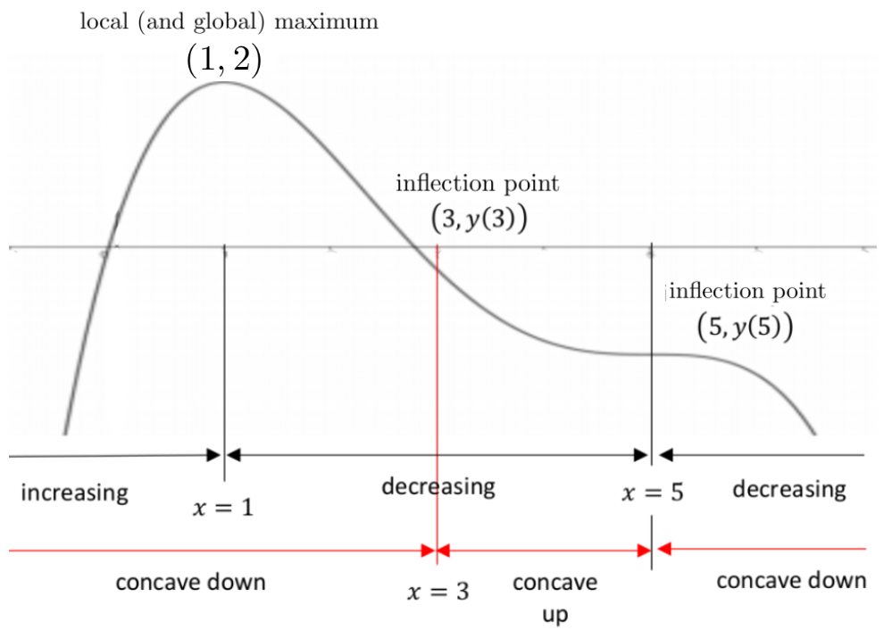
In a sense this is easier than the previous problems, since intervals of increase, decrease, concave up, and concave down have already been determined for us. For example, here are the tables for each.
In Example 10.2.1 we have \(\dfdxat{y}{x}{5}=0\) and \(\dfdx{y}{x}\lt 0\) on the intervals \((1,5)\) and \((5,\infty)\text{.}\) Given that \(\dfdxat{y}{x}{5}=0\) and \(\dfdxn{y}{x}{2}\lt 0\) when \(x\gt 5\text{,}\) did we really need to specify that \(\dfdx{y}{x}\lt0\) on the interval \((5,\infty)\text{?}\)
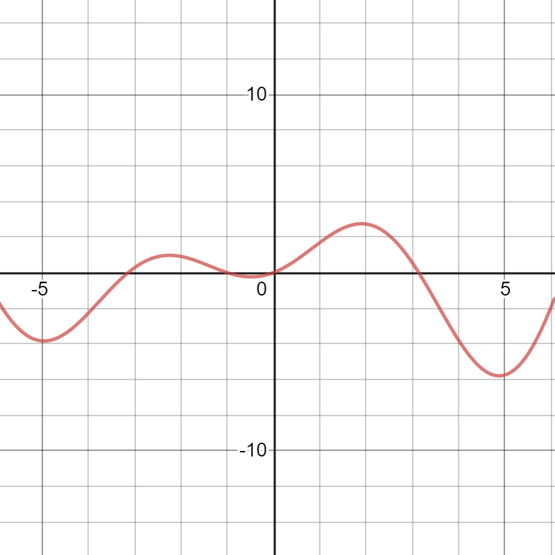
Based on the information given, the function \(y=y(x)\) has a local maximum at \(x=1\) and inflection points at \(x=3\) and \(x=5.\) A sketch of the graph might look something like this:
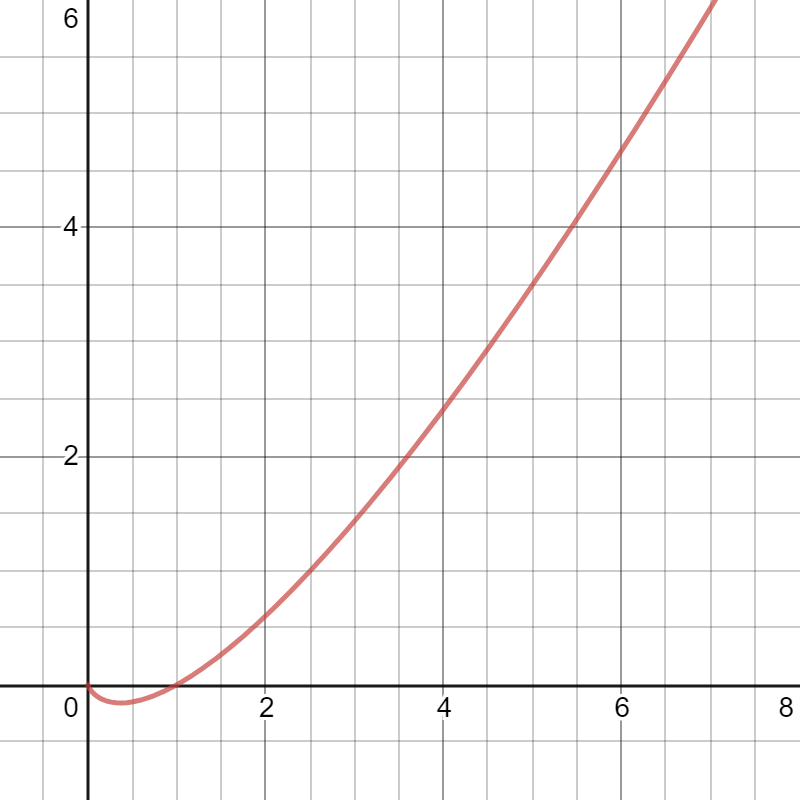
Subsection10.2.2Graphing \(y(x)\) from the Graph of \(\dfdx{y}{x} \)
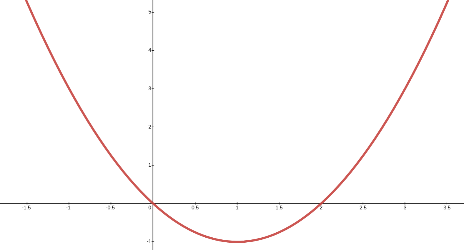
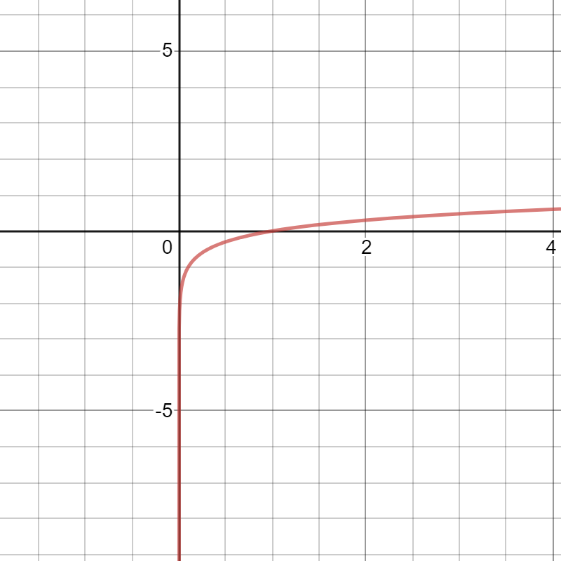
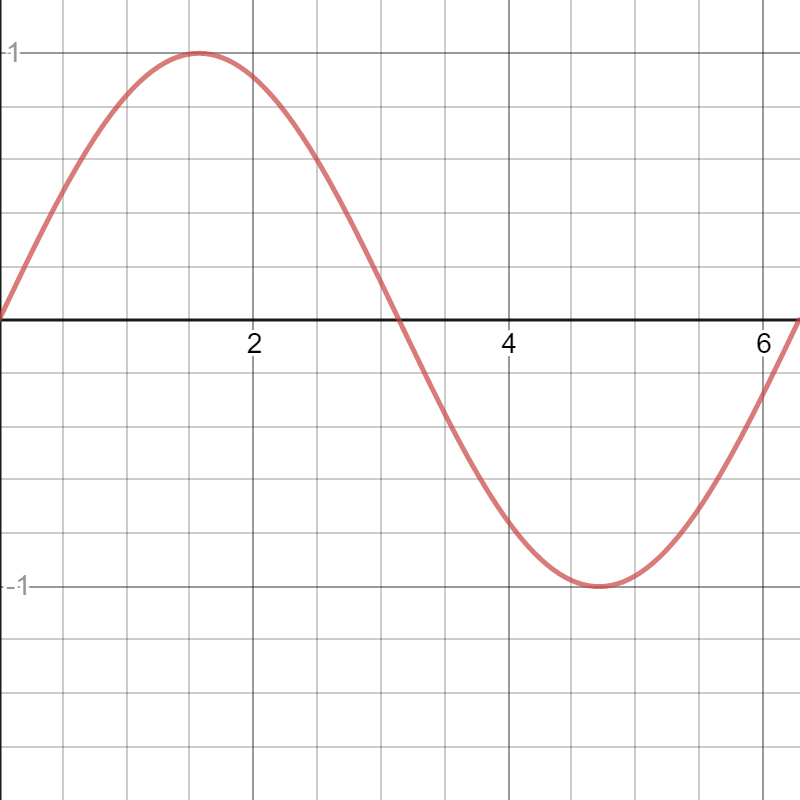
In Section 6.5 we found the graph of \(\inverse\tan(x)\) by examining the graph of its derivative, the Witch of Agnesi. The procedure we used in Section 6.5 is quite general. For example, suppose the graph of \(\dfdx{y}{x}\) is given below.
Recall that with a graph for \(\dfdx{y}{x}\text{,}\) finding where \(y\) is increasing or \(y\) is decreasing is just a matter of determining where the derivative is positive (above the \(x\) axis) or negative (below the \(x\) axis). Similarly the concavity of the graph of \(y(x)\) can be determined by finding where \(\dfdx{y}{x}\) is increasing (so \(y\) is concave upward) and decreasing (so \(y\) is concave downward). Equivalently, we find where \(\dfdxn{y}{x}{2} \) is positive and where it is negative. Given the graph of \(\dfdx{y}{x}\) above, we can produce the following tables.