
Section 10.3 Graphing with a Formula for \(\dfdx{y}{t}\)

Subsection 10.3.1 When \(\dfdx{y}{t}\) Depends on \(t\) alone

Example 10.3.1.

Consider the IVP,
\begin{align*} \dfdx{y}{t}=t(4-t), \amp{}\amp{} y(0)=0. \end{align*}
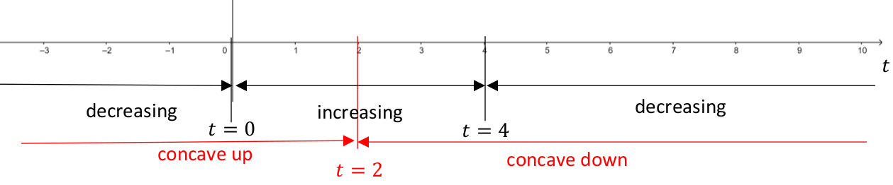
In Integral Calculus (probably your next math course) you will learn how to find \(y(t)\) explicitly. For now we will be satisfied with sketching an approximate graph of \(y(t)\text{.}\) Setting \(\dfdx{y}{t}=0\) and solving we see that \(t=0\) and \(t=4\) are the POTPs for \(y(t)\text{.}\) Thus on each of the intervals \((-\infty,0)\text{,}\) \((0,4)\text{,}\) and \((4,\infty)\) the graph of \(y(t)\) is either always increasing or always decreasing. We tabulate this information as follows:
Table 10.3.2. POTPs
Interval \((-\infty, 0)\) \((0,4)\) \((4,\infty)\)
\(y^\prime (t)\) \(y^\prime (t)\lt0\) \(y^\prime (t)\gt0\) \(y^\prime (t)\lt0\)
\(y (t)\) \(\searrow\) \(\nearrow\) \(\searrow\)
Based on this table, we can see that \(y(0)=0\) is a local minimum and \(y(4)\) is a local maximum. Observe that we have no way to determine the value of \(y(4)\text{.}\) All we can say is that the value of \(y(4)\text{,}\) whatever it is must be a local maximum.
We proceed in a similar fashion to determine concavity. The second derivative is
\begin{equation*} \dfdxn{y}{t}{2}=\dfdx{(t(4-t))}{t}=4-2t. \end{equation*}
Setting \(\dfdxn{y}{t}{2}=0\) and solving, we see that \(t=2\) is a PITP for \(y(t)\text{.}\) Making a table as before we have
Table 10.3.3. PITPs
Interval \((-\infty, 2)\) \((2,\infty)\)
\(y^\prime(t) \) \(y^\prime(t)\gt 0\) \(y^\prime(t)\lt 0\)
\(y(t)\) \(\bigcup\) \(\bigcap\)
Based on the table we see that the point \((2,y(2))\) is an inflection point. We want to make a reasonable sketch of the graph of \(y=y(t)\) based on this information. But we need to be careful. There is a lot of information in Table 10.3.2 and Table 10.3.3 and our graph needs to be consistent with all of it. So we first organize all of our conclusions by plotting the transition points (both optimal and inflective) on the \(t\) axis and identifying the intervals where \(y\) is increasing, decreasing, concave up, or concave down.
This information, along with the initial value, \(y(0)=0\) allows us to provide a reasonable graph of \(y(t)\text{.}\)
From the initial condition in the IVP we know that \(y(0)=0\) but we have no information about the vertical coordinate of any other point on the graph. Thus, from the given information the scale of this graph is unknowable. The graph above is reasonable because it is consistent with the data given in the IVP but that is all we can say about it.
This sort of graphical, qualitative analysis is the best we can do with the information we have but, as you see, we can glean a great deal of information about the “shape” of the graph of a function from its derivative alone.

Problem 10.3.4.

For each of the following IVPs:
  1. Find the intervals on which the graph of the solution is increasing and decreasing. Identify the locations of all local extrema.
  2. Find the intervals on which the graph of the solution is concave upward and concave downward. Identify the locations of all inflection points.
  3. Plot a reasonable sketch of the graph for \(y=y(t).\) Approximate transition points using the appropriate technology or Newton’s Method as necessary.
  1. \(\dfdx{y}{t}=t^2 (4-t),\text{ } y(0)=0\text{.}\)
  2. \(\dfdx{y}{t}=t^2 (4+t),\text{ } y(0)=0\text{.}\)
  3. \(\dfdx{y}{t}=\sin(t),\text{ } y(0)=0\text{.}\)
  4. \(\dfdx{y}{t}=\sin(t),\text{ } y(0)=2\text{.}\)
  5. \(\dfdx{y}{t}=\cos(t),\text{ } y(0)=0\text{.}\)
  6. \(\dfdx{y}{t}=\sin(t)\cos(t),\text{ } y(0)=\pi\text{.}\)
  7. \(\dfdx{y}{t}=t\sin(t),\text{ } y(0)=0\text{.}\)
  8. \(\dfdx{y}{t}=5e^t-t,\text{ } y(1)=1\text{.}\)
  9. \(\dfdx{y}{t}=-e^{-t}+\ln(t),\text{ } y(1)=e\text{.}\)
  10. \(\dfdx{y}{t}=e^t\sin(2t),\text{ } y(0)=1\text{.}\)
  11. \(\dfdx{y}{t}=\tan(t),\text{ } y(0)=1\text{.}\)
  12. \(\displaystyle \dfdx{y}{t}=\sqrt{t},\text{ } y(0)=1\)
  13. \(\displaystyle \dfdx{y}{t}=t^3-t,\text{ } y(1)=3\)
  14. \(\dfdx{y}{t}=t-t^3,\text{ } y(1)=3\)
    Compare this to problem (m).

Subsection 10.3.2 When \(\dfdx{y}{t}\) depends on \(y\) alone

            To see a World in a Grain of Sand
            And a Heaven in a Wild Flower
            Hold Infinity in the palm of your hand
            And Eternity in an hour
          
William Blake
 4 
https://www.poetryfoundation.org/poets/william-blake
(1757—1827)
Consider the IVP
\begin{align} \dfdx{y}{t}=y,\amp{}\amp{} y(0)=1.\tag{10.2} \end{align}
This is the same IVP we approximated in Section 7.3. The analysis we will do here is related so you may find it useful to review that section before proceeding.
As we’ve seen every IVP has two parts: a differential equation (in this case, \(\dfdx{y}{t}=y\text{,}\) and an initial value (in this case, \(y(0)=1\)).
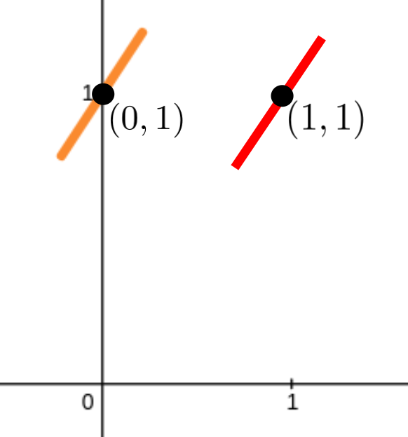
We will focus on the differential equation first. The differential equation \(\dfdx{y}{t}=y\) says that at each point on the graph of \(y(t)\) the slope of the graph is equal to the vertical coordinate at that point. For example if \((0,1)\) is a point on the graph of \(y(t)\text{,}\) then near that point the graph of \(y(t)\) will look like the orange part of the sketch below. On the other hand, if \((1,1)\) is a point on the graph of \(y(t)\) then near the point \((1,1)\) the graph of \(y(t)\) will look like the red graph in the sketch below.
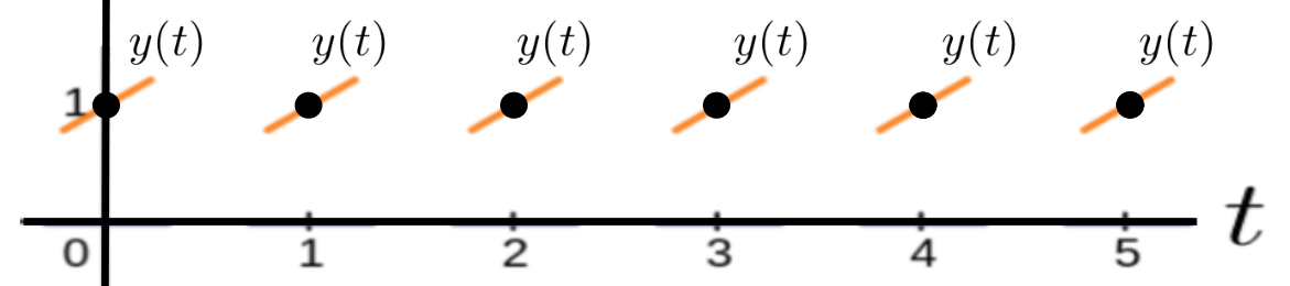
In fact, for any value of \(t\text{,}\) we know that if \((t,1)\) is a point on the graph of \(y(t)\) then the slope of the graph which passes through that point will be parallel to the orange and red lines above. That is, if a solution of the differential equation passes through a point \((t,1)\) then its slope will be equal to \(1\) at \((t,1)\) for any value of \(t\text{.}\)
This is seen in the figure below where each black dot represents a point with vertical coordinate equal to \(1\) and each orange segment represents the graph of the curve that both satisfies the differential equation from IVP (10.2), and passes through that point.
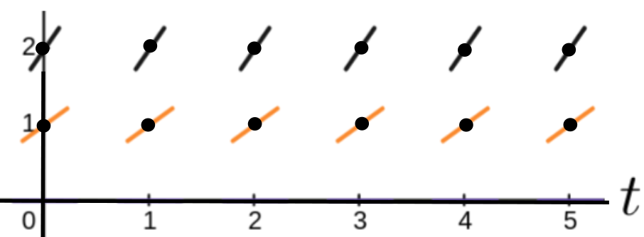
Similarly, if we know that \((t,2)\) is a point on the graph of \(y(t)\text{,}\) where \(y(t)\) both solves the differential equation from IVP (10.2) and passes through that point, then the slope at \((t,2)\) will be \(2\text{,}\) as seen in the following sketch.
By tagging more points in the plane in the same way we get the image below.
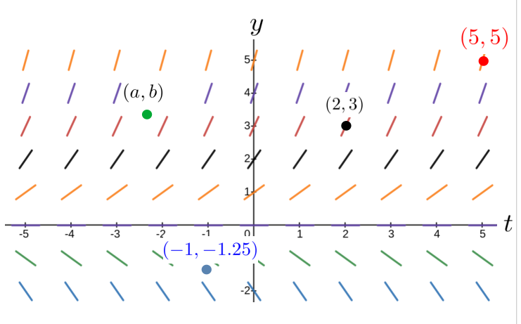
A sketch like this is called a slope field. The short line segment at each point, \((a,b)\text{,}\) is a short section of the graph of the function which satisfies the differential equation \(\dfdx{y}{t}=y\text{.}\)
If we know where to start (i.e., if we have an initial condition) the slope field allows us to determine the shape of the entire graph.
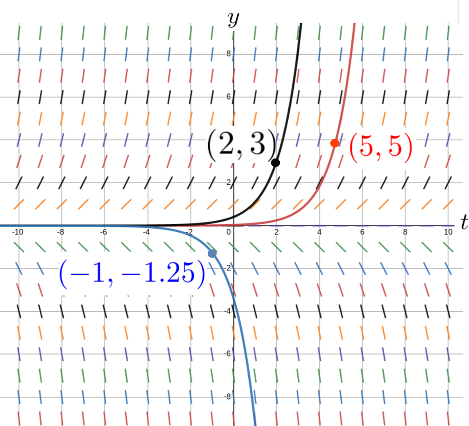
For example to sketch the graph of \(y(t)\) if it passes through the point \((2,3)\text{,}\) we simply follow the line segments in our slope field starting at that point. This is the black graph in the sketch below. The graph of the \(y(t)\) that passes through the point \((5,5)\) is shown in red below, and the graph that passes through the point \((-1,-1.25)\) is shown in blue.
Figure 10.3.5.

Drill 10.3.6.

IVP (10.2) has the initial condition, \(y(0)=1.\) Plot the point \((0,1)\) and use th slope field in Figure 10.3.5 to sketch the solution of IVP (10.2). Compare your solution with the approximation we obtained in Section 7.3. Do they look like the same solution?

Problem 10.3.7.

(a)
Confirm that \(y(t)=3e^{t-2}\) is the solution of the IVP
\begin{align*} \dfdx{y}{t}=y, \amp{}\amp{} y(2)=3. \end{align*}
(This is the black graph above.)
(b)
Confirm that \(y(t)=5e^{t-5}\) is the solution of the IVP
\begin{align*} \dfdx{y}{t}=y, \amp{}\amp{}(5)=5. \end{align*}
(This is the red graph above.)
(c)
Based on parts (a) and (b) guess what the solution of the IVP
\begin{align*} \dfdx{y}{t}=y, \amp{}\amp{}y(-1)=-2 \end{align*}
will be. Confirm that your guess is correct. {If you guess wrong, guess again.}
(d)
Based on parts (a) and (b), and (c) guess what the solution of the IVP
\begin{align*} \dfdx{y}{t}=y,\amp{}\amp{} y(a)=b \end{align*}
will be. Confirm that your conjecture is correct.
To sketch the graph of the solution of a given IVP begin by drawing the slope field for the differential equation. Then plot the value and follow the slope field to sketch the graph.

Problem 10.3.8.

For each of the following IVPs sketch the slope field in the ranges given and use your slope field to sketch the solution of the IVP.
(a)
\(\dfdx{y}{t}=\sqrt{y},\text{ }y(0)=1,\text{ }-5\le t, \text{ }y\ge0\)
Hint.
It is often simplest to begin by sketching slopes at integer coordinate points in order to get a clearer sense of the graphs. Then to fill in between them.
(b)
\(\dfdx{y}{t}=y^2,\text{ }y(-1)=-2,\text{ }-5\le t\le 5,\text{ }-5\le y\le 5\)
(c)
\(\dfdx{y}{t}=(y-1)^2,\text{ }y(1)=0,\text{ }-5\le t\le 5,\text{ }-5\le y\le 5\)
(d)
\(\dfdx{y}{t}=y(y-2),\text{ }y(1)=1,\text{ }-1\le x\le 1,\text{ }-2\le y\le 3\)
(e)
\(\dfdx{y}{t}=y(2-y),\text{ }y(1)=1,\text{ }-1\le t\le 1,\text{ }-2\le y\le 3\)
(f)
\(\dfdx{y}{t}=(y^2-1),\text{ }y(0)=1,\text{ }-2\le t\le 2,\text{ }-2\le y\le 2\)

Subsection 10.3.3 When \(\dfdx{y}{t}\) Depends on \(y\) and \(t\)

So far we’ve examined the situation when \(\dfdx{y}{t}\) depends on \(t\) alone:
\begin{equation*} \dfdx{y}{t}=f(t) \end{equation*}
and when \(\dfdx{y}{t}\) depends on \(y\) alone:
\begin{equation*} \dfdx{y}{t}=f(y)\text{.} \end{equation*}
But, of course, it could happen at \(\dfdx{y}{t}\) depends on both \(y\) and \(t\text{:}\)
\begin{equation*} \dfdx{y}{t}=f(t,y)\text{.} \end{equation*}
Analytically, this is a more complex situation but sketching the graph of the solution of such an IVP from its slope field is still possible.

Problem 10.3.9.

For each of the following IVPs draw The slope field in the ranges given and use your slope field to sketch the solution of the IVP.
(a)
\(\dfdx{y}{t}=ty,\text{ }y(0)=1,\text{ }-3\le t\le 3,\text{ }y\ge0\)
(b)
\(\dfdx{y}{t}=\frac{y}{t^2+1},\text{ }y(1)=0, \text{ }-5\le x\le 5,\text{ }-5\le y\le 5\)
(c)
\(\dfdx{y}{t}=ye^t,\text{ }y(-4)=2,\text{ }-5\le t\le 5,\text{ }-5\le y\le 5\)
(d)
\(\dfdx{y}{t}=ye^{-t},\text{ }y(0)=2,\text{ }0\le t\le 5,\text{ }-5\le y\le 5\)