One of the mathematicians who developed techniques for solving optimization problems was
Pierre de Fermat (1601–1665) who created what has been called the
Method of Adequalty. (The Latin root
adequāre means to equalize. When something is adequate, then it is equal to the need.) Fermat’s method was based on the simple observation that if the maximum value of
\(y\) occurs when
\(x\) is equal to say,
\(6\text{,}\) then when
\(x\) is very near
\(6\text{,}\) \(y\) will almost be equal to its maximum value.
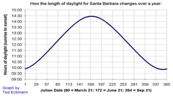
You can see this in the graph above. Notice that the maximum number of daylight hours (about
\(14.5\)) occurs just after
\(169\) days (in fact, at day
\(172\)) and that for several days before or after we have about the same number of hours of daylight. This is also true near the minimum which occurs at day
\(356\text{.}\) Regardless of what the variables represent if the graph of a function,
\(f(x)\text{,}\) is continuous then
\(f(x+h)\approx f(x)\) near a maximum or minimum: as long as
\(h\) is not too big.
Fermat’s simple idea was to purposely make the mistake of setting
\(f(x+h)\) actually equal to
\(f(x)\text{.}\) He then rearranged the formulas algebraically and at the crucial point he would set
\(h=0\) to “make it correct.” An example will make this clearer.
Example 3.4.3.
In
Example 3.3.4, we showed that out of all rectangles with a fixed perimeter, the one with the largest area is a square. Next we will use Fermat’s Method of Adequality to examine the related question: Out of all rectangles with a fixed area, does a square have the smallest perimeter?
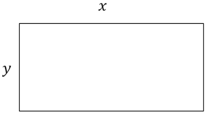
Consider a rectangle whose length is
\(x\) and whose width is
\(y\text{.}\) The area of the rectangle is given by
\(A=xy\) and the perimeter is given by
\(P=2x+2y\text{.}\)
The problem is to minimize \(P\) while holding \(A\) constant. More precisely, our objective is to minimize the function \(P=2x+2y\text{,}\) subject to the constraint that the area, \(A=xy\text{,}\) is fixed. First, we will use our constraint \(A=xy\) to eliminate one of the variables and substitute into \(P\text{.}\) Solving for \(y,\) we get \(y=A/x\text{.}\) Then,
\begin{equation*}
P=P(x) = 2x+\frac{2A}{x}.
\end{equation*}
We have used function notation for \(P(x)\) to emphasize that \(P\) is a function of \(x\) alone. (Remember that \(A\) is constant or “fixed.”)
Fermat’s method says to first set
\begin{equation*}
P(x+h)=P(x).
\end{equation*}
This gives:
\begin{gather}
2(\textcolor{red}{x}+h)+\frac{2A}{x+h}=2\textcolor{red}{x}+\frac{2A}{x}.\tag{3.1}
\end{gather}
Rearranging a bit, we get
\begin{align*}
\textcolor{red}{2x}+\textcolor{blue}{2}h+\frac{\textcolor{blue}{2}A}{x+h}\amp{}=\textcolor{red}{2x}+\frac{\textcolor{blue}{2}A}{x}
\end{align*}
so that
\begin{align*}
h\amp{}=\frac{A}{x}-\frac{A}{x+h}.
\end{align*}
Adding the fractions gives
\begin{align}
h\amp{}=\frac{A(x+h)-Ax}{x(x+h)}=\frac{Ah}{x(x+h)}. \tag{3.2}
\end{align}
Finally, and crucially, dividing both sides by \(h,\) gives
\begin{align}
1\amp{}=\frac{A}{x(x+h)}.\tag{3.3}
\end{align}
Earlier we had made the “mistake” of setting
\(P(x+h)=P(x)\) (knowing that this is not true). Now we “make it correct” by setting
\(h=0\text{.}\) This gives:
\(1=\frac{A}{x^2}, \text{ or } x^2=A. \) Substituting this into
\(y=\frac{A}{x},\) we get
\(y=\frac{A}{x}=\frac{x^2}{x}=x\text{.}\)
Thus
\(P\) is minimum when
\(y=x,\) which is to say, when the rectangle is actually a square. A moment’s thought should make it clear that there is no maximum value for
\(P\text{.}\)
Fermat’s method is very slick. However it contains an inherent logical flaw. We begin by setting
\(P(x+h)\) equal to
\(P(x)\text{,}\) even though we know we are making an error. This seems like it might be a flaw but it really isn’t. When we set
\(P(x+h)=P(x)\) we are asking, “What happens if they are equal?” The computations leading up to
equation (3.3) are the answer to that question.
But notice that we got from
equation (3.2) to
equation (3.3) by dividing by
\(h\text{.}\) But we know that we can only divide by
\(h\) if
\(h\) is not zero. Fortunately it is clear that
\(h\ne0\) since the whole point of introducing
\(h\) is for
\(x+h\) and
\(x\) to be two different values. However, in the final step, after
equation (3.3), we took
\(h=0\) to “make it correct” but if
\(h\) is zero then we couldn’t have divided by
\(h\text{.}\) We seem to be chasing our tails. We need for
\(h\) to be equal to zero and not be equal to zero at the same time!
This is the logical flaw.
Since we began with the assumption that
\(h\neq0\) we can’t just change our minds later. We can’t have both
\(h=0\) and
\(h\neq0\text{.}\)
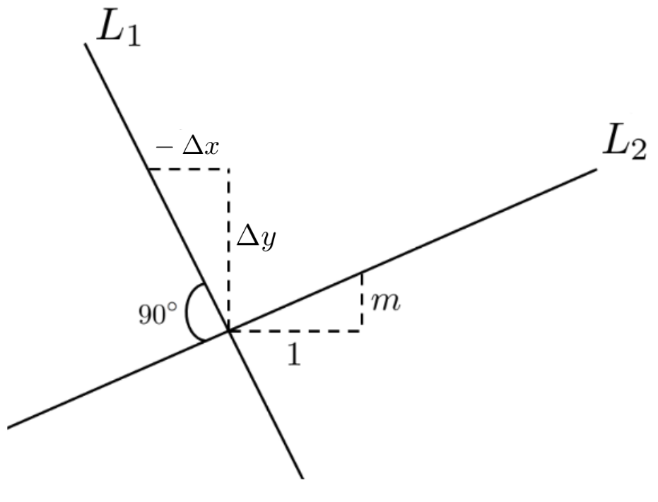
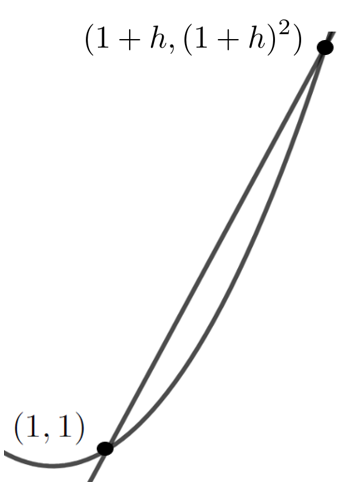
We need two points to determine the slope of a line, so with Fermat’s method in mind, we choose another point on the curve
\(y=x^2\) very close to
\((1,1)\text{.}\) Since we don’t really care which point we take as long as it is close to
\((1,1)\) we introduce the parameter,
\(h,\) which we think of as very small. The points
\((1,1)\) and
\((1+h,(1+h)^2)\) are thus very close together. This is represented in the sketch below.
The slope of secant line joining \((1,1)\) and \((1+h,(1+h)^2)\) is given by
\begin{align*}
\frac{(1+h)^2-1}{(1+h)-1}\amp{}=\frac{1+2h+h^2-1}{h}\\
\amp{}=2+h\text{.}
\end{align*}
As before we set \(h=0\text{.}\) Thus the slope of the line tangent to the graph of \(y=x^2\) at \((1,1 )\) is \(2\text{.}\)