Section8.8John Napier Logs In: A Short Introduction to Logarithms
In the \(16\)th and \(17\)th centuries the computational needs of science, engineering, finance and navigation were growing increasingly complex, time–consuming, and error prone. The problem of navigating at sea using only the stars as a guide was particularly vexing. It became increasingly important to find very accurate methods of computation that were also as simple as they could possibly be; that could be broken down into simple steps that anyone could do without necessarily understanding the underlying concepts. The Scottish mathematician John Napier devised one such method.
Napier described logarithms in Mirifici logarithmorum canonis descriptio (A Wonderful Description of the Canon of Logarithms), published in \(1614\text{,}\) well before Newton or Leibniz were born so logarithms actually predate the invention of Calculus by several decades. He coined the term “logarithm” from the Greek words logos meaning “reasoning,” or “reckoning” and arithmos meaning “number.” To Napier logarithms were “reckoning numbers” which seems an apt description, given their original purpose.
The crucial observation here is that exponentiation (raising to a power) takes the addition of the exponents \(n\) and \(m\) and turns it into the multiplication of \(a^n\) and \(a^m\text{.}\) Of course, multiplying instead of adding makes computations more complex, not less. This is exactly the reverse of what is needed. What Napier wanted was a way to turn the complexity of multiplication into the simplicity of addition. This would make complex computations -- especially computations done by hand with paper and pencil (the only kind there was in those days) much simpler.
Now the multiplication of \(a^n\) and \(a^m\) has become the addition (in the exponent) of \(n\) and \(m\text{.}\) Of course there is much more to be done to make this a usable computational scheme. But this is the essential idea. For example if we wanted to use this scheme to multiply \(123.2387\times 43.8378\) we would first need to know that \(123.2387 \approx 10^{2.0907}\) and that \(43.8378 \approx
10^{1.6418}\text{.}\) Adding the exponents gives \(3.7325\) so the result of the multiplication is \(10^{3.7325}\approx5401\text{.}\) The way to make this a workable scheme is to compile a large table of numbers and their associated exponents. This is, essentially, what Napier did.
Today we call \(2.0907\) and \(1.6418\) the base 10, or common logarithms, of \(123.2387\) , and \(43.8378\text{,}\) respectively. Notationally we have
In general, \(\log_{10}(10^n)=n\text{,}\) and we see that the function \(\log_{10}()\) simply undoes the function \(f(x) =
10^x\text{,}\) which makes \(\log_{10}()\) the functional inverse of \(f(x) = 10^x\text{,}\) in exactly the same way that \(\inverse\tan(x)\) is the functional inverse of \(\tan(x)\) as you saw in Section 6.4.
To use a table of base \(10\) logarithms to find the product of two numbers we would first look up the logarithm of each number, then add the logarithms. The resulting sum is the base \(10\) logarithm of the product, so we’d look up in our table what this sum is the logarithm of. The result is the product of the two original numbers. Since the invention of modern computing technology the original purpose of base \(10\) logarithms — simplifying numerical computations — is completely obsolete. So tables of base \(10\) logarithms are rarely seen in the wild anymore. On the other hand the natural exponential function \(\exp(x)=e^x\) and its functional inverse, the natural logarithm — usually denoted \(\ln(x)\) — are both still quite useful in a variety of contexts, both scientific and mathematical.
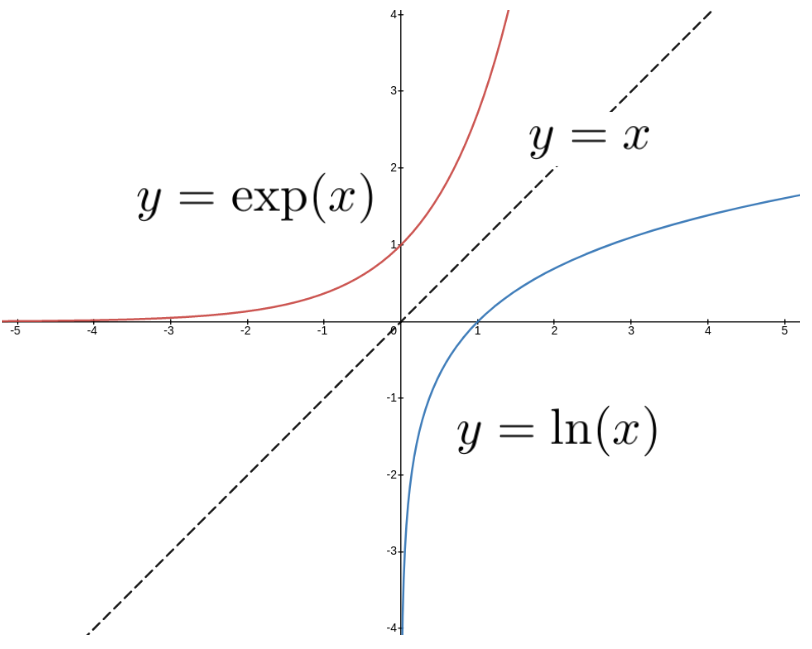
The graph of the natural exponential is very similar to the graph of \(y=3^x\text{.}\) As we saw in Section 6.4 if we have the graph of some function we can find the graph of its inverse by interchanging the horizontal and vertical axes. As a practical matter, this is the same as reflecting the graph across the line, \(y=x\text{.}\) The graph of the natural exponential and its inverse the natural logarithm are shown in Figure 8.8.2 below.
In the same way that \(\log_{10}(x)\) is the functional inverse of the base ten exponential, \(10^x\text{,}\) the natural logarithm is the functional inverse of the natural exponential, \(e^x\text{.}\) This inverse relationship allows us to immediately identify several important properties of the natural logarithm.
The properties that make the natural logarithm useful as a theoretical tool are the same properties that made \(\log_{10}(x)\) useful as a computational tool. In fact if we replace the base \(10\) with the base \(e\) and “\(\ln\)” with “\(\log_{10}\)” all of the properties in this list remain true.