Section5.9Self–intersecting Curves and Parametric Equations
In Problem 5.2.11 we asked you to find the line tangent to several interesting curves. However, we were careful to ask only about relatively simple curves. In particular, none of the curves in Problem 5.2.11 intersected themselves. We avoided self–intersecting curves earlier because we didn’t have the techniques necessary to address the problem of tangent lines at points where a curve crosses itself. We do now.
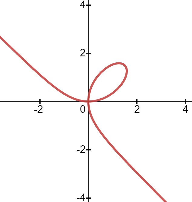
If we try to compute \(\eval{\dfdx{y}{x}}{(x,y)}{(0,0)}\) for the Folium of Descartes we find that \(\eval{\dfdx{y}{x}}{(x,y)}{(0,0)}=\frac{0}{0}\) which is very strange. We can see in the graph that at \((0,0)\) there is both a horizontal and a vertical tangent line, so it seems to make some sort of sense.
You might be thinking that we have stumbled upon a new rule about tangent lines: If we ever obtain \(\dfdx{y}{x}=\frac{0}{0}\text{,}\) at some point then the curve has both a vertical and horizontal tangent at that point. It would be nice if things were that simple, but they aren’t.
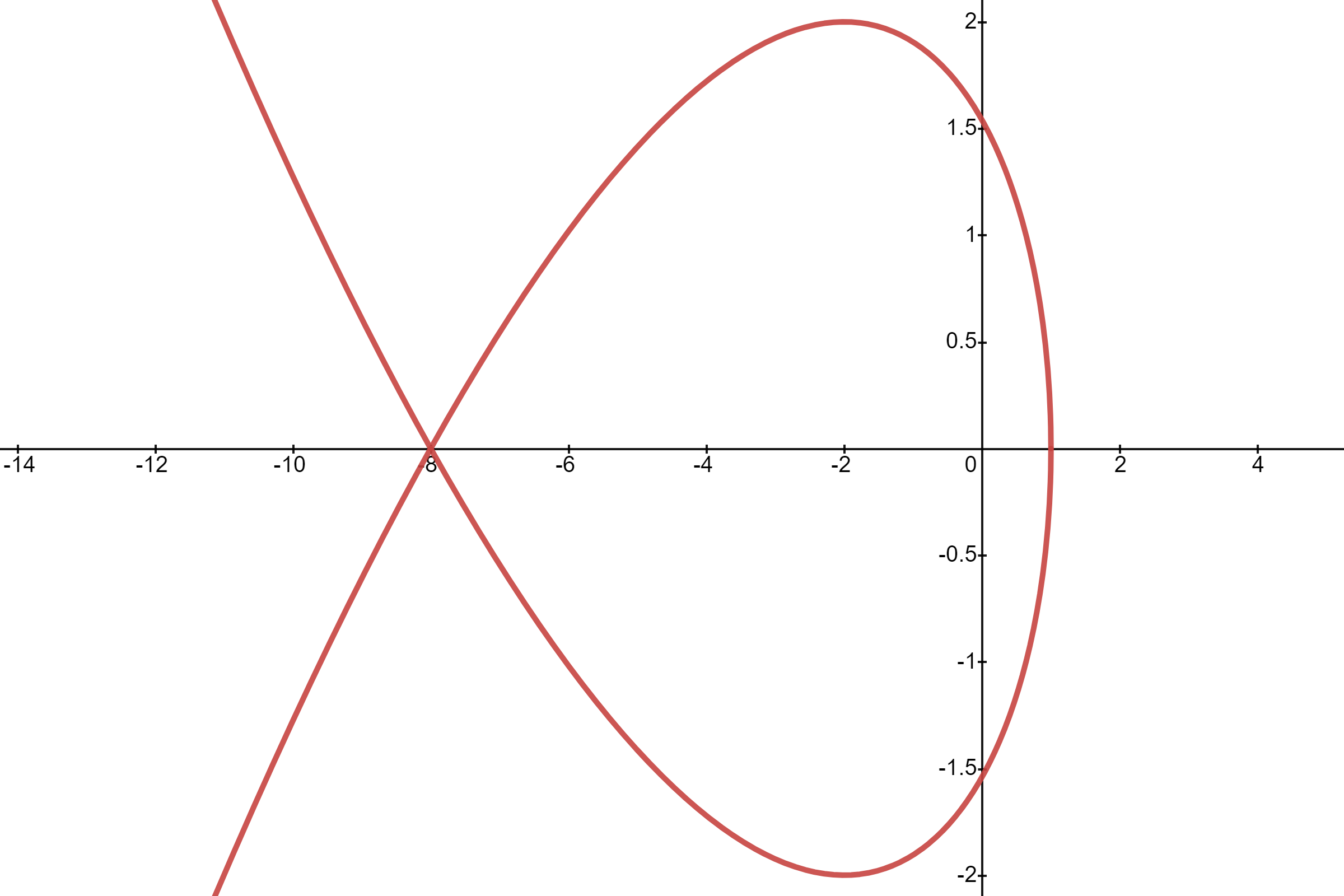
But now consider the Tschirnhausen Cubic at the self–intersection point \((-8,0)\text{.}\) As long as we stay away from the self–intersection point there are no difficulties. But from the graph we can see that any sort of tangent line at the point of self–intersection would be neither vertical nor horizontal despite the fact that once again we have
If nothing else, these examples illustrate that using Calculus is much more subtle than simply computing a derivative. A cavalier attitude can lead to some very strange anomalies. As is true of any powerful tool, to avoid disaster we must be careful.
The safest approach is to avoid points of self–intersection and fractions such as \(\frac00\text{.}\) But we won’t be able to avoid them forever so we might as well address the issue now. Adopting Newton’s dynamic approach will give us the crucial insight. Think of the horizontal and vertical coordinates as Newton’s fluents; things changing in time.
Using the static approach to find a tangent line at a self–intersection point is very much like standing in the center of the intersection of two roads and trying to decide if the road goes north–south or east-west. Obviously the road doesn’t go anywhere. It just sits there. Likewise, a curve is not dynamic. It just sits there, like a road.
If instead we ask, “Which way are we going as we pass through the intersection?” there is only one answer. We’re going in the direction we were traveling when we entered the intersection. If we think about the situation dynamically rather than statically, we always have both a position on the curve and a direction we are traveling.
If we are traveling along a curve our direction of travel is always tangent to the curve. By changing our question from “What is the tangent line at this point?” to “What is the tangent line at this time?” the concept of two (or more) tangent lines at a single point in space becomes meaningful. Each tangent is obtained by passing through the point of tangency at distinct moments in time.
If we think of \(t\) as time, with \(t\lt 0\text{,}\) representing time in the past, will the point \((x(t), y(t))\) traverse the clockwise or counterclockwise as \(t\) increases?
Find the values of \(t\) for which \((x(t), y(t)) = (-8,0)\text{.}\) Use the result of part (b) to compute \(\dfdx{y}{x} =\frac{\dot{y}}{\dot{x}}\) at these times. Are your answers consistent with what you obtained in part (c)? Explain.
Find the value of \(t\) for which \((x(t), y(t)) = (0,0)\text{.}\) use the result of part (b) to compute \(\dfdx{y}{x}=\frac{\dot{y}}{\dot{x}}\) at this time. Is this consistent with the graph?
What comes along with this change in interpretation is this: We no longer want to think of a differential ratio only as a slope. If \(y\) and \(x\) happen to represent the vertical and horizontal coordinates of a graph, then the change of \(y\) with respect to \(x\text{,}\)\(\dfdx{y}{x}\text{,}\) will be the slope of the curve \(y=y(x)\text{.}\)
If \(y\) represents the vertical position of an object and \(t\) represents the time when the object is at position \(y(t)\text{,}\) then the change of \(y\) with respect to \(t\text{,}\)\(\dfdx{y}{t}=\dot{y}\text{,}\) is the vertical velocity of the object as it passes through \(y\text{.}\) Likewise, if \(x(t)\) represents the horizontal position of an object then \(\dfdx{x}{t}=\dot{x}\) is the horizontal velocity of the object as it passes through \(x\text{.}\)
In general, if \(\alpha\) and \(\beta\) are two related quantities then \(\dfdx{\alpha}{\beta}\) is the rate of change of \(\alpha\) with respect to \(\beta\text{.}\) The physical (or geometric) interpretation of \(\dfdx{\alpha}{\beta}\) will necessarily depend on what \(\alpha\) and \(\beta\) represent physically (or geometrically).
When we switched to Newton’s dynamical viewpoint, we changed the nature of our representations of the curves. For example the Folium of Descartes can be represented by the formula as
\begin{equation*}
x^3+y^3=3xy.
\end{equation*}
This formula is complex and can be hard to work with, mainly because the relationship between \(x\) and \(y\) is difficult to see and understand.
the relationship between \(x\) and \(y\) is still difficult but since \(x(t)\) and \(y(t)\) are both functions the relationship between \(x\) and \(t\) and between \(y\) and \(t\) is a bit simpler. We know how to work with functions.
This second representation is usually called the parametric functions or parametric equation representation, because the \(x\) and \(y\) coordinates are given in terms of a parameter. In this case the parameter \(t\) represents time. This is common but by no means required. The parameter might represent anything, just as any variable might.
In fact, you might be wondering where we got the parameterization for the Folium. It may not seem obvious, but as long as \((x,y)\neq(0,0)\text{,}\) the parameter \(t\) actually represents the slope of the line joining the origin to the point \((x,y)\) on the Folium.
Let \((x,y)\) represent any point on the Folium \(x^3+y^3=3xy\) which is not the origin. Let \(t\) represent the slope of the line joining the origin to \((x,y)\text{;}\) that is, \(\frac{y}{x}=t\) or \(y=tx\text{.}\) Use this to show that
\begin{equation*}
x=\frac{3t}{1+t^3},\text{ and } y=\frac{3t^2}{1+t^3}.
\end{equation*}
The difference between this problem and Problem 5.9.3 is this: In Problem 5.9.3 we gave you \(x(t)\) and \(y(t)\) and asked you to show that it satisfies the equation of the Folium. Here we start with the equation of the Folium and you need to find \(x(t)\) and \(y(t)\text{.}\)
Of course, it is not wrong to also think of this parameter as time. We are just stipulating that the point is moving so that its position at time \(t\) is such that the slope of the line joining the origin to the point matches \(t\text{.}\) Mathematically, what the parameter represents is usually not at issue. It is just a parameter.
Recall that when we looked at Roberval’s treatment of the conic sections in Section 3.6 we found it handy to think of our curves as being traced out by the motion of a point and we created the notation \(\ParamEqTwo{x(t)}{y(t)} \) to reflect that point of view. With one slight modification this notation suits our current needs as well.
First, since the coordinates of our point are, individually, functions of \(t\) it follows that the position of the point \(P\) itself depends on (is a function of) \(t\) as well:
Second, it is useful for us to have a convenient way to specify the domain of the function. So we add a third component to do that. For example, if the domain of our function is all values of \(t\) strictly between zero and one we would write.
“Dynamic” and “static” are only words we use to describe the way we’re thinking about a problem. There is nothing inherently dynamic or static in either representation so there is no a priori reason to prefer one over the other. They describe the same set of points in the plane.
For example if \(y=x^2\) then \(\dx{y}=2x\dx{x}\text{.}\) Time (\(t\)) does not appear in these formulas so we tend to think of them statically. However if we want to think of them dynamically we divide by \(\dx{t}\) to get \(\dfdx{y}{t}=2x\dfdx{x}{t}\) and interpret this to say that at any given time \(t\text{,}\) the position of a point is \(\ParamEqTwo
{x(t)}
{y(t)}\) and the vertical velocity, \(\dfdx{y}{t}\) is twice the value of the \(x\) coordinate times the horizontal velocity, \(\dfdx{x}{t}\text{.}\)
The parameterization \(P(t)=
\ParamEqThree
{-(t^2+1)}
{t^4+2t^2+1}
{-\infty\lt t\lt \infty}\) traces out different part of the same parabola. How else is this parameterization different from the one in part (a)?
Moving between the equation and parametric forms can be very hard to do depending on the complexity of the equation. The simplest situation is when you have \(y\) as a function of \(x\text{;}\) for example \(y(x)=x^2\text{.}\) To find a parametric representation we observe that we need to specify both \(x\) and \(y\) as functions of a third parameter, \(t\text{.}\) This can be puzzling until we realize that \(x\) is completely free. All we need to do is ensure that \(y=x^2\text{.}\) So if we take \(x(t)=t\) and \(y=x^2=t^2\) we almost have our parameterization.
When faced with a formula like \(y=x^2\) you have learned to always assume that \(x\) could be any real number that makes sense in the formula. But with parametric equations this assumption can lead to problems. We’ll need to specify the allowable values of the parameter \(t\) explicitly. This is why we said we almost have our parameterization. A complete parameterization must specify the values of \(t\) that are available to us, so in this case
We can always parameterize the graph of a function the same way we just parameterized \(y=x^2\text{.}\) A parameterization of \(y=y(x)\text{,}\) with domain \(a\le x\le b\) is
Sketch only the part of the curve included in each parameterization in part (a). Be sure to indicate the direction of travel in each case, assuming \(t\) is increasing.
As we’ve seen we can always parameterize the graph of a function, but the reverse is not true. A parameterized curve will not always be the graph of some function. For example the curves in Problem 5.2.11 are not graphs of functions, but all of these curves can be parameterized.
Because it can’t always be accomplished there is no general strategy for expressing a parameterized curve as the graph of a function. One strategy that sometimes works is to find \(\dfdx{y}{x}\) and “undifferentiate” as in the following example.
Show that the point \(\left(1,0\right)\) is on our parameterized curve. Use this to find the function, \(y(x)\text{,}\) that has the same graph as \(P(t))\text{.}\)