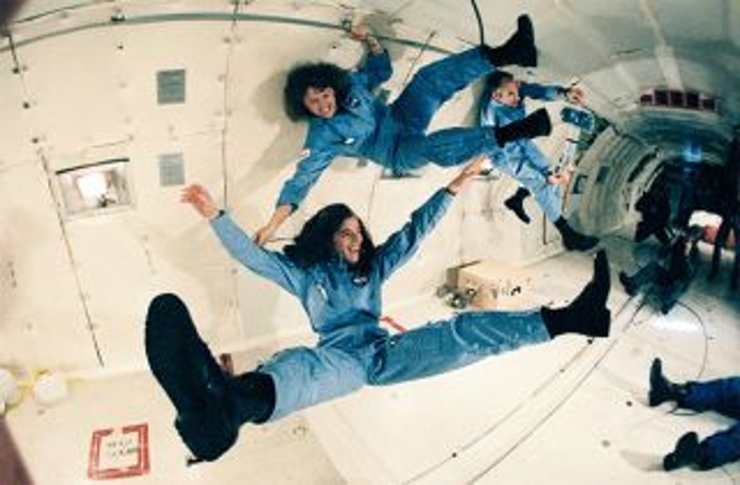
To acclimate astronaut trainees to the effects of weightlessness, NASA has an airplane perform a series of steep climbs and sharp dives. At the top of each climb passengers will experience weightlessness for about \(25\) seconds. During a training flight the pilot will repeat this maneuver about \(40\) times.
Because this “roller coaster” ride sometimes causes nausea for the passengers the planes used for the maneuver have been christened “Vomit Comets.” One of these airplanes was used to film the weightless scenes in the \(1995\) film Apollo 13.
It is well known that the path of an object moving only under the influence of the Earth’s gravity at the surface of the earth is parabolic. To simulate weightlessness inside the plane the Vomit Comet is flown so that its flight path matches such a parabolic flight. That is, its shape will be the graph of a curve having the form
We’d like to find the values of the unknown parameters \(A\text{,}\)\(B\text{,}\) and \(C\) that match the path of an object moving under the influence of Earth’s gravity. Once these are known we will also be able to determine the peak altitude of the flight and how far (horizontally) it will go before coming back to the altitude where the maneuver began. That is, we can find the point where the pilot should enter, and later exit, the parabolic flight. Finally we’d like to confirm the claim that this maneuver takes about \(25\) seconds.
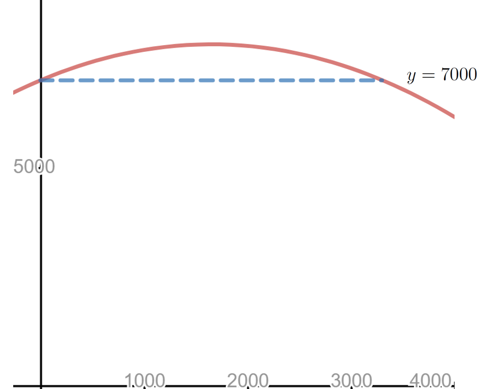
Suppose the following graph depicts the parabolic flight path followed by the Vomit Comet as it starts its maneuver at an altitude of \(7000\) meters and an initial angle of elevation of \(45^\circ\text{.}\)
To find \(A\text{,}\) we’ll need to have a better model of the motion. Fortunately, Calculus is exactly the right tool for building such a model but we don’t yet have all of the pieces we need. We will return to the Vomit Comet problem once we have them.
The pilot of a Vomit Comet seeks to simulate weightlessness, but the pilot of a commercial airliner works hard to avoid subjecting its passengers to extreme effects like weightlessness or, at the other end, of extreme gravity. So an airliner must descend more gradually. This situation is a little easier to understand so we will explore it in the next couple of problems and examples before returning to the Vomit Comet.
A fundamental tenet of mathematically modeling real world phenomena is to keep things as simple as possible. So, the first thing we’d be likely to try for is a parabolic descent path:
\begin{equation*}
y=Ax^2+Bx+C.
\end{equation*}
But it is pretty clear that this won’t work because the plane should be traveling horizontally at the beginning and at the end of its descent. At the end, because at that point it should be on the ground, and at the beginning because we don’t want to terrify the passengers.
Show that there is only one point on any parabola where the line tangent to the curve is horizontal. Explain why this proves that the flight path of the airliner in Example 5.3.2 cannot be parabolic.
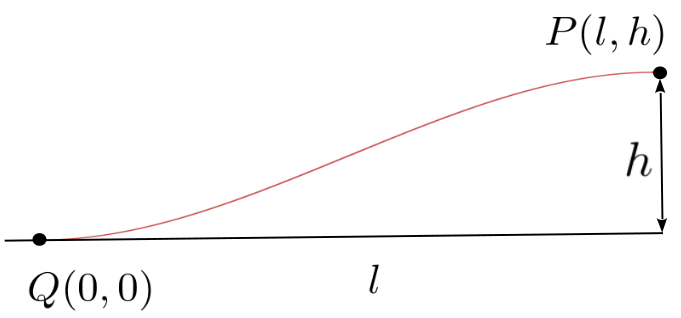
Below is a section of a cubic polynomial depicting a flight path with the plane starting initially at the point \(P(l,h)\) and ending at the airport \(Q\) which we will arbitrarily designate as the origin.
We’ve taken our analysis of the flight paths of both the Vomit Comet and our airliner as far as we can using slopes alone. The problem is that a flight path is like a road. A road doesn’t go anywhere. It just sits there. But an object traveling along a road (or a flight path) is moving. It has a velocity and an acceleration.
Analyzing a static path does not allow us to model either the velocity or the acceleration of an object moving along that path. Fortunately for us, Newton’s dynamic view of Calculus is just the tool we need to attack these problems. We will return to them in Section 5.7.
Since the Vomit Comet aims to replicate the path of a body falling freely under the influence of gravity we will also need to understand the influence of gravity on the motion of bodies. We address this in the next section.