Suppose we start with a colony of \(10\) grams of bacteria in a Petri dish and we wish to model the growth of the population as a function of time. In order to keep our initial discussion simple we begin by assuming that \(30\%\) of our bacteria divide once per day at the same time. Such a population is growing at a rate of \(30\%\) per day. If we start with \(10\) grams of bacteria on day zero, then on day one we’ll have \(30\%\) more, or \(13\) grams. On day two we’ll have \(30\%\) more than on day one, or \(16.9\) grams. It should be clear that the rate of growth from day \(n\) to day \(n+1\) is proportional to how many bacteria we have on day \(n\text{.}\) Thus from any one day to the next we see that the change in \(P\) (that is, \(\Delta P\)) is given by
\begin{equation}
\Delta P = 0.3 P\Delta t\tag{8.17}
\end{equation}
where \(\Delta t = 1\) day, and \(\Delta P\) is the change in population on that day.
But we assumed that \(30\%\) of the bacteria were dividing in sync once per day, which is unrealistic. To get closer to reality suppose next that enough of them divide during any one hour so that at the end of one day the population has still grown by \(30\%\text{.}\) Then from any one hour to the next we again have equation (8.17) but this time \(\Delta t\) is equal to one hour, or \(\frac{1}{24}\) day. However, we don’t have to measure time in days. If we measure it in hours instead we again have \(\Delta t=1 \text{ hour } = \frac{1}{24} \text{ day}\text{.}\) The constant factor is still \(0.3\) because we assumed that the population was growing at \(30\%\) per day, and this is still true. That factor is called the nominal growth rate.
If we measure time in seconds the same reasoning will give us equation (8.17), with \(\Delta t=1 \text{ second } = 1.15741\times 10^{-5} \text{
day}\text{.}\) If we measure in nanoseconds we get equation (8.17), with \(\Delta t=1 \text{ nanosecond } = 1.15741\times 10^{-14}
\text{ day}\text{.}\) If we measure time in infinitesimal increments we get
Notice that we are once againusing the Principle of Local Linearity 5.2.5 here. In this infinitesimal time interval the nominal growth rate, \(0.3P \text{,}\) is virtually constant and so we are treating it as linear growth.
Since we started with \(10\) grams of bacteria we have the initial condition \(P(0)=10\text{.}\) This says that the amount of bacteria at time \(t\) must satisfy the IVP:
Take specific notice that the differential equation in IVP (8.18) expresses the idea that the rate of change of the population, \(\dfdx{P}{t}\text{,}\) is proportional to the size of the population, \(P\text{,}\) and that the constant of proportionality is \(0.3\text{,}\) or \(30\%\text{.}\)
Clearly there is nothing particularly special about the number \(0.3.\) If our colony had been increasing at a nominal rate of \(15\%\) we’d have arrived at the IVP
From Problem 8.6.2 we see that a solution of the differential equation in our bacterial growth problem, IVP (8.18), is \(\rho(t)= e^{0.3t}\text{.}\) But \(\rho(t)\) does not satisfy the initial condition since
Show that if \(\alpha\) is any constant then \(P(t)=\alpha e^{0.3t}\) solves the differential equation \(\dfdx{P}{t}=0.3P\text{.}\) What is \(P(0)\text{?}\)
Did your answer in part (c) account for the possibility that \(\alpha=0\text{?}\) If not, redo it assuming that \(\alpha=0\text{.}\) What is \(P(t)\) in this case?
Suppose our growth rate was \(15\%\) per day. Would the bacteria have grown half as much in the first day as it did when the growth rate was \(30\%\) per day?
In general, if we start with a population of, say \(P_0\text{,}\) and the rate of change of \(P(t)\) is proportional to \(P\) itself then it will satisfy an IVP of the form:
The constant \(r\) is called the nominal growth rate as we’ve seen. Because \(r=\frac{\dfdx{P}{t}}{P}\) it is also called the relative growth rate of the population and is often given as a percentage, as we have done here.
The IVP (8.19) should look familiar to you. Notice that when \(r=1\) and \(P_0=1\) it is the same as IVP (8.2) which we used to define the the natural exponential. Except, of course, for the names of the variables. To put it another way IVP (8.19) is the special case of IVP (8.2) when \(r=1.\) Since these are so similar it is not surprising that the solution of IVP (8.19) involves the natural exponential.
Part 8.6.4.c indicates that there are limitations to the usefulness of IVP (8.18) and its solution, \(P(t)=10e^{0.3 t}\text{.}\) If we use it to predict how much bacteria there would be after one year we get \(P(365)=10e^{0.3\times365}\approx3.59\times10^{48}\) grams. Since current estimates of the mass of the entire universe are around \(6\times10^{27}\) grams, it is pretty clear that our model doesn’t work in the long term.
Clearly the bacteria can not sustain a growth rate of \(30\%\) indefinitely. If nothing else, they will eventually run out of food. Our point here is that this model, like all models, is limited. To use a mathematical model effectively we need to stay within its limitations.
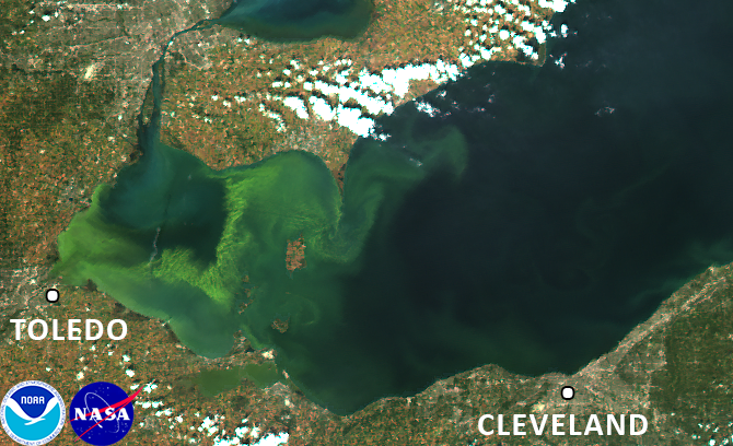
The green discoloration on the western side of the lake is from an explosive (exponential) growth of algae. When the conditions for algae growth are nearly optimum — if there is abundant food, there is room for the population to expand into, and the water temperature is exactly right — the population of algae in Lake Erie tracks with our model nearly perfectly. The quantity of algae grows exponentially until the conditions become sub-optimal. Then the population of algae drops again to normal levels.
An algal bloom can happen in any body of water where algae grow. They are common in alpine lakes in the early spring when nutrients are released by the melting snow, but the fish and insects that feed on the algae have not yet emerged in large numbers. We will return to this problem in Section 11.1 where we will tweak this model to extend its usefulness to longer periods of time. But for now we will continue to use this exponential growth model with the understanding that for large values of \(t\) it is unreliable.
Suppose our bacteria population is increasing at a relative rate of 10% per day. If we started with 100 grams, how much would there be after one, two, and three days?
Speaking loosely, the observation that lead us to IVP (8.19) is that the number of baby bacteria in a given generation is proportional to the number of mama and papa bacteria were present in the previous generation. Speaking very loosely, more parents now, means proportionally more babies later. This is all that is required for exponential growth to occur.