Were he alive today Michel Rolle might be horrified to know that his lemma has become a fundamental part of the modern development of Calculus. Like Bishop Berkeley, he was an early critic of Calculus, having once described it as a “collection of ingenious fallacies.”
Suppose \(f\) is continuous on the closed interval \([a,b]\) and differentiable on the open interval \((a,b)\text{.}\) Suppose further that \(f(a)=f(b)\text{.}\) Then there is at least one number \(c\text{,}\) in the interval \((a,b)\) such that \(f^\prime(c)=0\text{.}\)
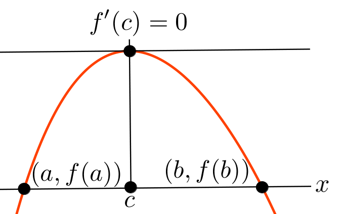
When Rolle’s Lemma is visualized, as in the sketch above, it is clear what is going on. If \(f(a)=f(b)\) then between the points \((a,f(a))\) and \((b,f(b))\) the graph of \(f(x)\) will either rise to a maximum or drop to a minimum (not shown) at some point \(c\text{.}\) In either case, by Fermat’s Theorem, the derivative of \(f\) at \(c\) will be zero. Notice that the slope of the line through \((a,f(a))\) and \((b,f(b))\) is also zero. Thus these two lines are parallel.
Despite the clarity of our sketch, an analytic proof is still required because our sketch does not capture all of the possible ways that Rolle’s Lemma can manifest. This is demonstrated in Problem 15.2.3 below.
Sketch the graph of a function (different from the one in our sketch) which satisfies all of the conditions of Rolle’s Lemma and convince yourself that the conclusion of Rolle’s Lemma must still be true.
Show that the condition that \(f\) is continuous on \([a,b]\) is necessary by sketching the graph of a function which violates only that condition and the conclusion of Rolle’s Lemma.
Show that the condition that \(f\) is differentiable on \((a,b)\) is necessary by sketching the graph of a function which violates only that condition and the conclusion of Rolle’s Lemma.
By the Extreme Value Theorem 9.5.21 there are points \(\alpha\) and \(\beta\) in the interval \([a,b]\text{,}\) such that \(f(\alpha)\) is a global maximum, and \(f(\beta)\) is a global minimum. There are two possibilities for \(\alpha\) and \(\beta\text{:}\)
In this case since \(f(a)=f(b)\) the global maximum and the global minimum are equal. The only way that can happen is if the function is constant on the interval \([a,b]\text{,}\) and if \(f\) is constant then \(f^\prime(x)=0\) for every \(x\) in the interval \((a,b)\text{.}\) So we take \(c\) to be any point in \((a,b)\text{.}\)
In this case by Fermat’s Theorem, either \(f^\prime(\alpha)=0\text{,}\) or \(f^\prime(\beta)=0\text{.}\) So we take \(c=\alpha\) or \(c=\beta\) as appropriate.
DIGRESSION: Theorems and Lemmas, What’s the Difference?
Aside:Mathematical Terminology.
The distinction between a theorem and a lemma is very slight and rather arbitrary. Typically we call a statement a theorem if it is important and requires proof. We call it a lemma if it requires proof itself, and is used to simplify the proof of a theorem. This is not a hard-and-fast rule by any means. Sometimes we first prove a lemma as an aid to proving a theorem, only to find that the lemma is actually more important. However, having been originally dubbed a lemma the result is known ever after as a lemma. For example, in the present instance we will be using the Extreme Value, and Fermat’s Theorems to prove what often called Rolle’s Lemma, and then use use Rolle’s Lemma to prove the Mean Value Theorem. Then we will use the Mean Value Theorem to prove the First Derivative Test. It is all very chaotic.
Suppose \(f(x)\) is continuous on some closed interval, \([a,b]\text{,}\) and \(f\) is differentiable on \((a,b)\text{.}\) Then there is at least one number \(c\) in the open interval \((a,b)\) such that
The Mean Value Theorem (visualized in Figure 15.2.5 below) says that there is a point \(c\text{,}\) in the interval \((a,b)\) such that the tangent line at \(c\) and the line through \((a,f(a)\) and \((b,f(b))\) are parallel. Thus in the special case where \(f(a)=f(b)\) the Mean Value Theorem reduces to Rolle’s Lemma. In other words the Mean Value Theorem is a generalization of Rolle’s Lemma.
We said we would use Rolle’s Lemma to prove the Mean Value Theorem. To do that we’ll need to create a function -- we’ll call it \(\phi(x)\) — that satisfies all of the conditions of Rolle’s Lemma. If \(L(x)\) is the function whose graph is the line through \((a,f(a)\) and \((b,f(b))\) we see that
satisfies all of the conditions of Rolle’s Lemma 15.2.2. Therefore, by Rolle’s Lemma there is a point \(c\text{,}\) between \(a\) and \(b\) such that \(\phi^\prime(c)=0\text{.}\) Therefore
As we mentioned at the beginning of this chapter in French the Mean Value Theorem is known as the théorème des accroissements finis, literally the “theorem of the finite increments.”
To see why this is an accurate description let \(y=f(x)\text{.}\) Then \(f(b)-f(a) = \Delta y\) and \(b-a=\Delta x\text{.}\) So we can re-express equation (15.3)) as \(\Delta y=f^\prime(c)\Delta x\text{.}\) In this form it is clear that the Mean Value Theorem relates the finite increments \(\Delta y\) and \(\Delta x\) to the instantaneous rate of change \(f^\prime(c)\text{.}\)
The English name, “Mean Value Theorem” comes from interpreting the derivative as an instantaneous velocity. If \(t\) represents time and \(p(t)\) represents position at time \(t\text{,}\) then \(\frac{p(b)-p(a)}{b-a}\) is the average velocity in the time interval \([a,b]\text{.}\) Since \(p^\prime(c)\) is instantaneous velocity at time \(c\text{,}\) the conclusion of the Mean Value Theorem is that at some point in that interval, instantaneous velocity must match average (mean) velocity. For example, if you travel \(50\) miles in one hour then your average velocity is \(50\frac{\text{miles}}{\text{hour}}\text{.}\) But it is unlikely that you traveled at exactly \(50\frac{\text{miles}}{\text{hour}}\) for the entire hour. However, at one instant (possibly more) you had to have been traveling at exactly \(50\frac{\text{miles}}{\text{hour}}\text{.}\) This is the Mean Value Theorem. It provides the bridge we need to get from infinitesimals to finite intervals.