Section 7.4 Higher Derivatives, Lagrange, and Taylor
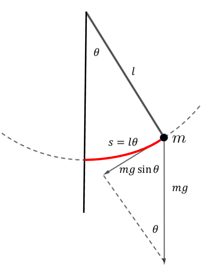
In the diagram below we see a pendulum of length \(l\) with an object of mass \(m\) at the end. If the object is moved away from its equilibrium point the pendulum will begin to swing back and forth. If we disregard friction the angle \(\theta\text{,}\) that the pendulum forms with a vertical line would oscillate in a manner very like the motion of the Simple Harmonic Oscillators (SHO) that we saw in Section 6.2.5.
If the motion of the pendulum actually is an SHO then it will necessarily satisfy equation (6.9). In this case that means that
\begin{equation*}
\dfdxn{\theta}{t}{2}=-\omega^2\theta,
\end{equation*}
for some constant value of \(\omega\text{.}\) We’ll investigate to see if that is true.
To keep our model simple we assume that \(-\pi\lt \theta \lt \pi\) and we will ignore any sort of resistance. The only force we are considering is the (vertical) force due to gravity \(mg\text{.}\) As before this vertical force will resolve into the centripetal force along the length of the pendulum, and the tangential force in the direction of motion. We will focus our attention on the tangential force.
If \(\theta\) is measured in radians then the length of the arc traced by the object is \(s=l\theta\text{.}\) Thus we see that the tangential component of the force due to gravity is given by \(mg\sin(\theta)\) as shown. Notice that when \(\theta\gt 0\) this tangential force points down and to the left and when \(\theta\lt 0\) it points up and to the right (not shown). This says that the sign of the tangential force \(F\) is the opposite of the sign of \(\theta\text{.}\) When \(\theta\) is in the interval \([-\pi, \pi]\) \(\theta\) and \(\sin(\theta)\) have the same sign. Thus We have \(F=-mg\sin(\theta)\text{.}\) Using Newton’s Second Law, \(\text{Force} = \text{mass}\cdot\text{acceleration}\text{,}\) we see that the motion of a pendulum satisfies the equation
\begin{equation*}
m\dfdxn{s}{t}{2}=-mg\sin(\theta).
\end{equation*}
Finally, since \(s=l\theta\) we have \(\dfdxn{s}{t}{2}=\dfdxn{(l\theta)}{t}{2}\text{.}\) Using the Constant Rule (twice) we see that \(\dfdxn{s}{t}{2}=l\dfdxn{\theta}{t}{2}\text{.}\) Thus
\begin{equation}
\dfdxn{\theta}{t}{2}=\frac{g}{l}\sin(\theta).\tag{7.8}
\end{equation}
The presence of \(\sin (\theta )\) shows that equation (7.8) does not have the same form as equation (6.9). Therefore a swinging pendulum is not a Simple Harmonic Oscillator. Its motion is slightly more complex.
But only slightly.
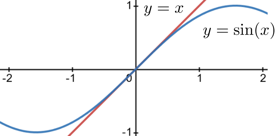
By examining the graphs of \(y=\sin(x)\) and \(y=x\) we can see the that for values of \(x\) close to zero the graphs are nearly identical. Thus, when the angle \(\theta\) is very small \(\sin(\theta)\) and \(\theta\) are very nearly equal. In that case if we replace \(\sin(\theta)\) with \(\theta\) in equation (7.8) we see the the motion of a pendulum approximately satisfies the equation
\begin{equation}
\dfdxn{\theta}{t}{2}=-\frac{g}{l}\theta,\tag{7.9}
\end{equation}
which we recognize as equation (6.9) with \(\omega^2 =
\frac{g}{l}.\)
Approximating \(\sin(x)\) by its tangent line at \(x=0\) works well for values of \(x\) close to zero. We have not been very precise about the meaning of “close to zero” but it should be clear that if \(\theta\) is too large equation (7.8) will no longer serve as a good model.
Notice that the function \(y(x) = x\) is a first degree polynomial. Is it possible that a polynomial with a higher degree will give us a better approximation? Can we find a polynomial with degree greater than one that approximates the graph of \(y=\sin(x)\text{?}\)
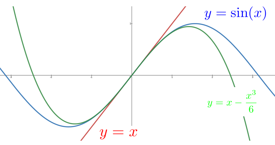
In the sketch below we compare the graphs of \(y=x\) (in red), \(y=\sin(x)\) (in blue), and \(y=x-\frac{x^3}{6}\) (in green) on the same set of axes. It should be clear \(y=x-\frac{x^3}{6}\) is a better approximation to \(y=\sin(x)\) than \(y=x\) in the sense that the graph of \(y=x-\frac{x^3}{6}\) stays closer to the graph of \(y=x\) on a wider interval than the graph of \(y=x\text{.}\)
So it seems reasonable to suppose that the differential equation
\begin{equation}
\dfdxn{\theta}{t}{2}=-\frac{g}{l}\left(\theta-\frac{\theta^3}{6}\right),\
\theta(t)=0,\tag{7.10}
\end{equation}
if we can solve it, would serve as a better model for the motion of a pendulum than equation (7.9). Unfortunately we do not yet have the tools to solve equation (7.10), but the notion of approximating a complex function, like \(\sin(x)\text{,}\) with a polynomial will turn out to be very useful so we will explore it for a bit before we go on. We will again switch to Lagrange’s prime notation because in this context Lagrange’s notation really shines. Indeed, it was while he was looking at similar problems that Lagrange invented his prime notation in the first place.
The key is to look at higher derivatives of \(\sin(x)\text{.}\) Recall that for \(y=f(x)\text{,}\) Lagrange introduced the notation and terminology
\begin{align*}
\dfdx{y}{x}\amp = f^\prime(x) \text{ (first derivative)}\\
\end{align*}
Extending this further, we have
\begin{align*}
\dfdxn{y}{x}{2} =\amp f^{\prime\prime}(x)=f^{(2)}(x) \text{
(second derivative)}\\
\dfdxn{y}{x}{3} =\amp f^{\prime\prime\prime}(x)=f^{(3)}(x) \text{ (third derivative)}\\
\dfdxn{y}{x}{4} =\amp f^{\prime\prime\prime\prime}(x)=f^{(4)}(x) \text{ (fourth
derivative)}\\
\amp \vdots
\end{align*}
Problem 7.4.2.
Show that the equation of the line tangent to the graph of an arbitrary (differentiable) function \(f(x)\) at \(x=0\) is given by
\begin{equation*}
y(x)=f(0)+f^\prime(0)\cdot x.
\end{equation*}
Applying the result of Problem 7.4.2 to \(f(x)=\sin(x)\) we see that the equation of the line tangent to the graph of \(y=\sin(x)\) at \((0,0)\) is given by
\begin{equation*}
y(x) = \sin(0)+\cos(0)\cdot x = x.
\end{equation*}
Problem 7.4.3.
This problem demonstrates how we can obtain a first degree polynomial that approximates \(f(x_0)\) near \(x=0\text{.}\) Suppose that \(f(x)\) is some (differentiable) function and that \(l(x) =A+Bx\text{.}\)
(a)
(b)
Next, suppose we want to find a second–degree (quadratic) polynomial, \(q(x)\text{,}\) for which \(f(0)=q(0)\text{,}\) \(f^\prime(0)=q^\prime(0)\) and \(f^{\prime\prime}(0)=q^{\prime\prime}(0)\text{.}\) It is clear that we can simply extend what we did in the previous problem. That is, we start with a generic second–degree polynomial, \(q(x) = A+Bx+Cx^2\text{.}\)
First we insist that \(f(0)=q(0)\text{.}\) Evaluating both functions at \(x=0\) gives
\begin{equation*}
f(0) =\eval{A+B x+C x^2}{x}{0} = A+B\cdot 0+C \cdot0^2 =A,
\end{equation*}
so \(A=f(0)\text{.}\)
To obtain \(B\text{,}\) differentiate both functions and insist that the first two derivatives of \(f(x)\) and \(q(x)\) match at \(x=0\text{.}\) That is,
\begin{equation*}
f^\prime(0)=\eval{\dfdx{q}{x}}{x}{0}
=\eval{B+2Cx}{x}{0}= B.
\end{equation*}
So \(f^\prime(0)=B\text{.}\)
Problem 7.4.4.
(a)
Differentiate again and set the second derivatives at \(x=0\) equal to one another to show that
\begin{equation*}
C= \frac{f^{\prime\prime}(0)}{2}.
\end{equation*}
(b)
Show that if the cubic \(c(x)=A+Bx+Cx^2+Dx^3\) has the same third derivative as \(f(x)\) at \(x=0\) then
\begin{equation*}
D=\frac{f^{\prime\prime\prime}(0)}{3\cdot2} = \frac{f^{(3)}(0)}{3\cdot2}.
\end{equation*}
(c)
Show that if the quartic \(q(x)=A+Bx+Cx^2+Dx^3+Ex^4\) has the same fourth derivative as \(f(x)\) at \(x=0\) then
\begin{equation*}
E=\frac{f^{(4)}(0)}{4\cdot 3\cdot2}.
\end{equation*}
It seems clear that we could use this procedure in a “machine–like” way to produce a polynomial approximation of any degree. In fact, this “machine” for producing approximating polynomials was known long before Lagrange, but he made it more tractable by replacing differentials and differential notation, which are very cumbersome to use here, with derivatives and his prime notation. In general this approximating polynomial is called a Taylor Polynomial after the English mathematician Brook Taylor (1685–1731), but was known to mathematicians before Taylor (including Newton and Leibniz).
Problem 7.4.5.
The process in Problem 7.4.4 is how we generated our cubic approximation to the sine function just before equation (7.10). In this problem you will replicate and extend that computation.
(a)
(b)
Find the fourth degree Taylor Polynomial approximation for \(f(x)=\sin(x)\text{.}\)
(c)
Find the fifth degree Taylor Polynomial approximation for \(f(x)=\sin(x)\) and graph both functions on the same set of axes.
(d)
Find the sixth degree Taylor Polynomial approximation for \(f(x)=\sin(x)\text{.}\)
Problem 7.4.6.
Find the second and fourth degree Taylor Polynomial approximations for \(f(x)=\cos(x)\) and graph them all on the same set of axes. Would it make any sense to use the fifth–degree Taylor Polynomial in this case? Explain.
In general the Taylor Polynomial of degree \(n\text{,}\) that approximates a differentiable function \(f(x)\) near zero is given by:
\begin{equation}
T(x)=y(0) +\frac{y^{\prime}(0)}{1!}x
+\frac{y^{(2)}(0)}{2!}x^2+\frac{y^{(3)}(0)}{3!}x^3
+ \cdots +
\frac{y^{(n)}(0)}{n!}x^n.\tag{7.11}
\end{equation}
As you might imagine Taylor Polynomials are incredibly useful approximation tools. At this point we have given you only the most basic of introductions. You will see this again in much more depth in the next course, Integral Calculus.
