In a time when women had very few options in life, Maria Gaëtana Agnesi(1718–1799) was both exceptional and very lucky. Her brilliance and talent were recognized early and nurtured by her wealthy father, who encouraged her studies and provided her with the best possible tutors to develop her talents. She mastered the Calculus of Newton and Leibniz and in \(1748\) wrote a series of textbooks on the topic titled Instituzioni Analitiche ad Uso Della Gioventù Italiana ( Analytical Methods for the use of Italian Youth). It was immediately recognized as a masterpiece of mathematical exposition and was used throughout Europe during eighteenth century. It was by far the most popular Calculus textbook in use at the time. An Englishman, John Colson (1690–1760), was so impressed with Agnesi’s work that in 1760 he took it upon himself to learn Italian specifically so that he could translate her text into English.
In her text, Agnesi collected many of the known results of the time and organized them for the instruction of students. The Latin name of one of the curves that she used for instruction is versoria (“rope that turns a sail”) because of its shape. Agnesi correctly translated this into Italian as “la versiera.” Unfortunately Colson mistook this for “l’aversiera” which means “witch.” As a result this particular curve has been known ever since as the Witch of Agnesi.
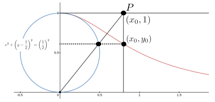
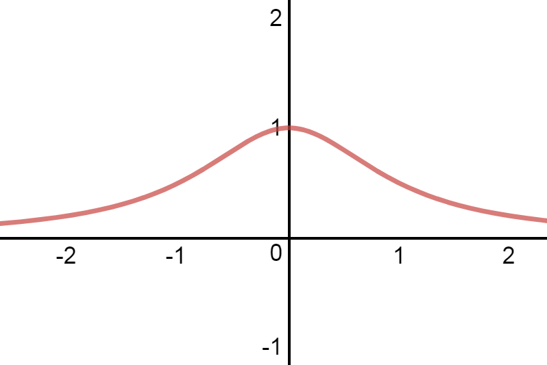
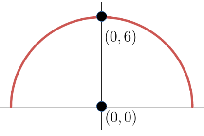
As modern function notation was yet to be invented Agnesi understood this curve geometrically as a particular set of points. In the diagram below think of \(P\) as moving from left to right along the line \(y=1\text{.}\) For each value of \(x_0\text{,}\) draw the line from the origin to \(P\) and locate the vertical coordinate \(y_0\) where this line intersects the circle
centered at \(\left(0, \frac12\right)\text{,}\) with radius \(r=\frac12\text{.}\) Every point \((x_0,y_0)\) is a point on the Witch of Agnesi. The Witch itself is the curve shown in red.
In the diagram above show that the coordinates \(x_0\) and \(y_0\) satisfy the equation, \(y_0=\dfrac{1}{1+x_0^2}\text{.}\) Thus the Witch is the graph of
Whenever you encounter a new curve an important question to ask is, “What is its derivative?” In this case you already have everything you need to find the answer.
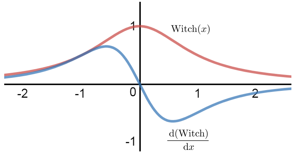
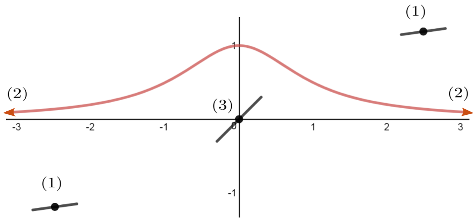
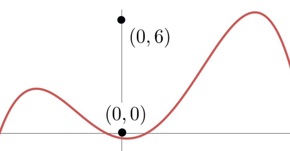
Computing the derivative of a function as a formula is very useful. This has in fact been our primary focus so far in this text. However to truly understand the relationship between a function and its derivative nothing can replace seeing both of them graphed together. Look closely at the relationship between the Witch and its derivative in the sketch below. Is it clear how these graphs are related?
Notice in particular that when \(x=0\) the \(y\) coordinate of the Witch is at its highest point (maximum value), whereas the \(y\) coordinate of \(\dfdx{(\text{Witch})}{x}\) is zero.
We know that the derivative of a curve at a given point gives us the slope of the line tangent at that point. Thus at the highest point of the Witch the line tangent to it will be horizontal. That is, the derivative of the Witch will be zero. This is exactly what these two graphs are showing us.
When \(x\) is just to the right of zero, the slope of the Witch is close to zero and negative. Similarly just to the left of zero the slope of the Witch is close to zero and positive. At the extreme right end of the graph above the slope of the Witch is close to zero and negative and at the extreme left it is close to zero and positive. And all of this is reflected in the shape of the blue (derivative) curve.
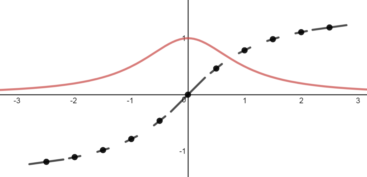
It is a little more interesting to reverse this process. That is, suppose we could see only the derivative of the Witch (blue curve). Could we figure out the shape of the Witch from this?
Consider: From the extreme left of the graph to \(x=0\) the \(y\)–coordinate of the (blue) derivative curve is above the \(x\)–axis. Therefore the slope of the Witch is positive. Clearly wherever the slope of a function is positive the function is increasing, so we can deduce that the Witch increases from left to right until we reach \(x=0\) where the blue derivative function crosses the \(x\)–axis.
Thereafter the \(y\)–coordinate of the blue derivative curve is below the \(x\)–axis. That is, the slope of the Witch is negative, so the Witch is decreasing.
Just by looking at the derivative curve we can see that the Witch of Agnesi increases from left to right until we reach \(x=0,\) and after that it decreases. Although this shows us the shape of the Witch we do not have enough information to completely describe the Witch of Agnesi. We can tell a lot about a curve by looking at the graph of its derivative but we can’t tell everything.
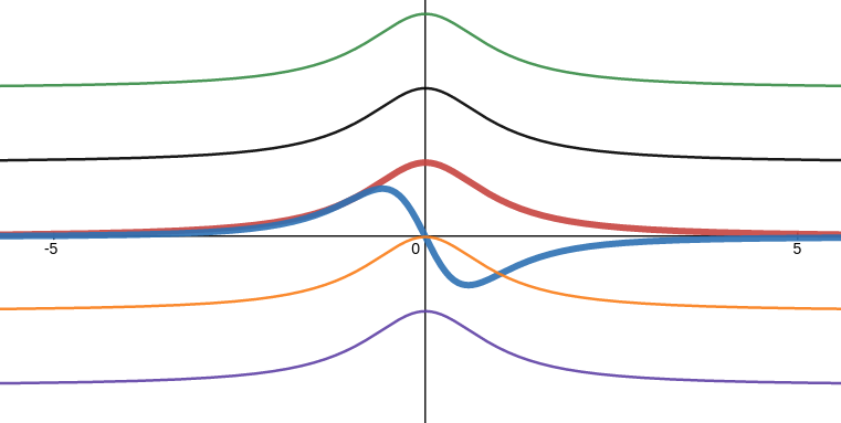
In the sketch below the red curve is the graph of the Witch and the blue curve is the graph of its derivative. Convince yourself that the blue curve could also be the graph of the derivative of any of the other curves shown as well. As clearly as you can, explain what this suggests about the relationship between a function and its derivative.
Next we’d like to apply this same sort of reasoning to the Witch itself. We’d like to answer the question, “What curve is the Witch of Agnesi the derivative of?” Whatever that curve is, we’ll call it the antiderivative of the Witch for obvious reasons.
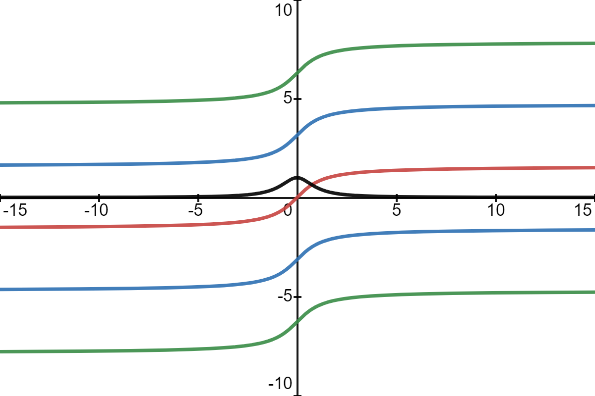
As before, by simply looking at the graph of the Witch we can see that: (1) At the extreme ends of its graph the antiderivative will have a positive slope which gets closer and closer to zero as we go farther from the origin, but (2) since the Witch never crosses the \(x\)–axis the antiderivative will never have a horizontal slope, and (3) at \(x=0\) the slope of the antiderivative will be equal to one. A sketch of the antiderivative of the Witch begins to emerge when we put these three observations into our graph:
We’ve been a little lazy with our use of language. As we saw in Problem 6.5.4, the antiderivative is not unique, so it is improper to speak of the antiderivative. Any one of the curves shown below could be an antiderivative of the Witch of Agnesi. (Except the black one, of course. That’s the Witch.)
This graph should look very familiar to you. It looks very much like the graph of the arctangent function we discussed in Section 6.4, doesn’t it? Do you suppose it is possible that the derivative of the arctangent function is the Witch of Agnesi?
Of course it is. Why else would we have led you down this path? But there are some subtleties here that we shouldn’t ignore. For example we will want to find a function that is the antiderivative of the Witch. We will proceed cautiously.
The following problem is not directly related to the Witch of Agnesi. We include it so that you can get practice relating the graphs of functions, their derivatives, and their antiderivatives, as this is a very useful skill. We will need it in a far more substantial way in Section 10.2 when we get there.
Sketch the graph of the the antiderivative passing through the point \((0, 0)\text{,}\) and of the derivative each of the following curves on the same set of axes,