Intuitively speaking, the curvature of a plane curve is how quickly a curve turns. It is an important property to understand when designing, for example, a road or a roller–coaster where the sharpness of a curve determines the safe speed limit for that curve. Also, the stresses imposed on the physical structure of a moving object during any high speed maneuver are directly related to the curvature of their paths.
One of the first people to study the notion of curvature was Nicole Oresme (1323–1382). Oresme defined the curvature of a straight line to be zero (no surprise), and he defined the curvature of a circle to be the reciprocal of its radius. For example, a circle with radius \(2\) is \(\frac12\) whereas the curvature of a circle with radius \(1\) is \(1\text{.}\) This makes intuitive sense. A circle with a smaller radius is “more curved” than one with a larger radius. The radius of the earth is so large that the curvature of say, the equator, is so close to zero as to be completely imperceptible, at least for someone standing on the surface.
Oresme’s definition of curvature works just fine for circles and straight lines but we’d like to extend it to more general curves. Specifically, given a curve, we’d like to associate a number with each point on the curve which tells us the curvature at that point. Ideally, this should also generalize Oresme’s results for straight lines and circles.
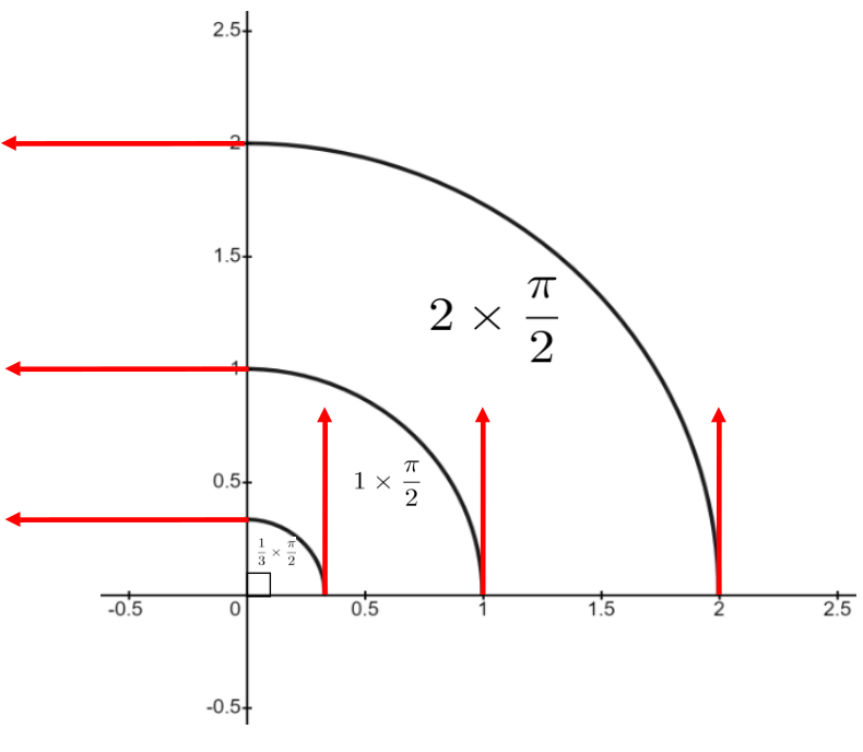
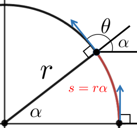
The sketch above shows three circles in the first quadrant with radii, \(\frac13\text{,}\)\(1\text{,}\) and \(2\text{,}\) respectively. Notice that on the unit circle, the point of tangency travels \(\frac{\pi}{2}\) units along the circumference while the the red tangent line rotates through an angle of \(\frac{\pi}{2}\) radians. On the circle of radius \(2\text{,}\) the point of tangency travels \(2 \times \frac{\pi}{2}\) units to turn the tangent line the same \(\frac{\pi}{2}\) radians, whereas on the circle of radius \(1/3\text{,}\) the point of tangency travels \(\frac13\times\frac{\pi}{2}\) units to turn the tangent line the same \(\frac\pi2\) radians. This suggests that a possible definition for curvature might be the number of radians the tangent line rotates through as it travels along the curve divided by the distance traveled along the curve while making the turn. In other words, the curvature for a circle of radius \(r\) would be
\begin{equation*}
\frac{\theta \text{ radians }}{r\theta \text{ units}}=\frac{1}{r}
\text{ radians per unit. }
\end{equation*}
This seems to make intuitive sense too. A circle with a radius of \(0.0000001\) meters certainly seems to be “more curved” than a circle with radius \(1,000,000,000\) meters.
This definition works fine for circles and straight lines which have constant curvature, but what about a more general curve. What if the curvature changes from point to point along the curve such as a long and winding road.
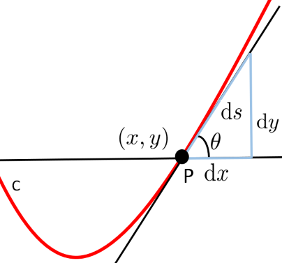
Clearly we’ll need a definition of curvature that also changes from point to point on the curve. So it seems reasonable to consider infinitely small changes in both the angle \(\theta\) and in arclength \(s\text{.}\) More precisely, we make the following definition.
It can be difficult at first to see how formula (6.19) measures curvature but think carefully for a moment about the meaning of the expression \(\dfdx{\theta}{s}\text{.}\) Loosely put “the rate of change of \(\theta\) (the angle of our curve with the horizontal) with respect to the change of \(s\) (the arclength of our curve)” is the ratio of how much a point moving on the curve has changed direction to how far it has moved. The more our curve changes direction in a given distance the more it is curved and so the more curvature it has.
Don’t let the absolute value bars in this formula disturb you. They are there simply because we don’t want to consider whether a curve bends to the right or to the left (whether \(\theta\) is increasing or decreasing), but just how fast it bends.
A good test of the value of a new definition is whether or not it produces the same results that earlier, more intuitive musings led us to. It should be clear that with this definition, the curvature of a straight line is zero (Why?) just like Oresme’s definition.
In Problem 6.8.4 it was helpful to know that the line tangent to a circle is always perpendicular to its radius. But for an arbitrary curve this is not necessarily true. Let’s look at the general situation.
First recall from equation (6.20) that \(\tan(\theta) = \dfdx{y}{x}\text{.}\) Rewrite this as \(\theta=\inverse\tan\left(\dfdx{y}{x}\right)\) and differentiate so that
The time has come for us to begin understanding why differentials were abandoned as a foundational concept for Calculus. We are entering dangerous and uncharted waters but we won’t dive into the deep part just yet. We’ll only wade in a little way.
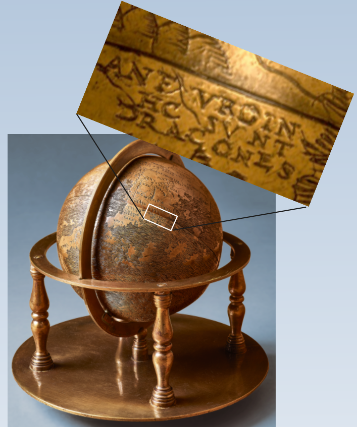
To indicate dangerous and uncharted waters on their maps medieval mapmakers would fill in the unexplored regions of their maps with illustrations of dragons and other mythological beasts. The Lennox Globe, in the Rare Book Division of the The New York Public Library (1510 CE), even has the inscription Hic Sunt Dracones (Here Be Dragons) along the eastern Asian coast.
If the entire development from equation (6.21) to equation (6.24) feels contrived, it’s because it is contrived. In particular the “uncancelling” step is clearly a trick in the sense that nothing we did before that step seems to motivate the uncancelling. We just pulled it out of the air, and it worked. Clearly we knew that it would work, but why do you suppose we used a trick rather than explaining what we were doing?
Since everything we did hinged on the observation that \(\dfdxn{y}{x}{2}=\dfdx{\left(\dfdx{y}{x}\right)}{x}\) (from equation (6.23) and equation (6.24)) it would seem more natural to simply apply the Quotient Rule to \(\dx{\left(\dfdx{y}{x}\right)}\text{,}\) wouldn’t it?
But the expressions \(\dx(\dx{x}) =\dx^2x\) and \(\dx(\dx{y}) =\dx^2y\) are a problem because to get equation (6.24) when we are finished we need to have \(\dx^2x =0\text{,}\) but \(\dx^2y\neq0\text{,}\) which seems inconsistent. Why would \(\dx^2y\) be something, but \(\dx^2x\) be nothing? This is very troubling.
We have observed regularly beginning in Chapter 4 that the concept of a differentials is questionable. But if differentials are problematic, second differentials — differentials of differentials — are even moreso, if that is possible.
When we use Leibniz’ differential notation we think of \(\dx{y}\) and \(\dx{x}\) as infinitesimal increments in the \(x\) and \(y\) coordinates. Specifically, \(\dx{x}=x_2-x_1\) where \(x_2\) and \(x_1\) are infinitely close together. This is already a difficult thing to accept.
But if we stick with Leibniz then it must be that \(\dx(\dx{x})
= \dx{x_2}-\dx{x_1}\text{,}\) right? We can write this down and we can read these symbols easily enough. But what they seem to mean is that \(\dx(\dx{x})\) is the infinitely small difference of two infinitely small differences. So does that mean that \(\dx(\dx{x})\) just another differential? Or is \(\dx(\dx{x})\) smaller than \(\dx{x}\text{?}\) But \(\dx{x}\) is infinitely small so how could \(\dx(\dx{x})\) be smaller than that?
For Newton, time was the only variable, and time always flows forward at a constant rate. He thought of a variable, \(x\) for example, as moving, or flowing (fluent) in time and \(\dot{x}\) was the rate of flow (fluxion) of the fluent\(x\text{.}\) In the simplest example, if \(x\) is the position of a point then \(\dot{x}\) is its velocity.
Newton only applied his dot notation to something that was changing in time; something that has a rate of change with respect to time. Can we apply it to time itself?
Sure we can. Time itself is “changing in time”, isn’t it? Time flows at a rate of \(1\) second per second, or one day per day, or one century per century. The units don’t really matter. Loosely speaking (and mixing the Newtonian and Leibnizian viewpoints a bit), an increment of time now has the same magnitude as an increment of time later, has the same magnitude as an increment of time in the past. That is, every increment of \(t\) is the same size. If we let \(t\) represent elapsed time then this means that the infinitesimal increment \(\dx{t}\) is constant, so the fluxion of \(\dx{t}\) is zero:
that this is not true of a quantity that is flowing at a variable rate. For example, if \(y=t^2\) then \(\eval{\dx{y}}{t}{1}=2\dx{t}\) whereas \(\eval{\dx{y}}{t}{2}=4\dx{t}\text{.}\)
Moreover we always have the option of adopting Newton’s convention that the only independent variable is time so that when we write \(\dfdx{y}{x}\) we are thinking of the independent variable \(x\) as time (although we rarely say so out loud), and we are thinking of \(y\) as functionally dependent on time (represented by \(x\) in this case). Therefore
\begin{align*}
\dx^2x=\dx(\dx{x})=0
\amp{}\amp{}\text{ and } \amp{}\amp{}
\dx^2y=\dx(\dx{y})\neq0.
\end{align*}
As a practical matter we will rarely be interested in second order differentials like \(\dx^2x\) or \(\dx^2y\text{.}\) As we indicated in Section 4.1 the notion of a differential is really just an aid to computation, a convenient fiction. Differentials are a helpful aid but the more important and useful concept is the derivative. Differentials only serve as a step along the way to finding derivatives.
On the other hand, we will be very interested in second order derivatives: \(\dfdx{\left(\dfdx{y}{x}\right)}{x} =
\dfdxn{y}{x}{2} \) because these often represent a real, physical quantity like force or acceleration.
But now there is another difficulty that can’t be ignored. In order to make sense of the expression \(\dx^2{x}\) we had to abandon Leibniz’ conception altogether. It is nice that Newton’s viewpoint gives us a way to make sense of the notation but what this tells us is that taking either viewpoint (Newton’s or Leibniz’) does not get us to the logical heart of the matter. A viewpoint is just a manner of thinking. We adopt a viewpoint in order to build intuition.
When two viewpoints are at odds it means that we need something deeper and more general. In this case we need a theory that subsumes, and can replace, the views of both Leibniz and Newton. This issue must, eventually, be addressed. But for now we will continue to work intuitively. When we are done, when we stand at the top of the Calculus mountain we will be able to see the paths that Newton and Leibniz each took to get to the top. We will begin our own trek to the summit in Chapter 13.
Since the equation of a straight line is \(y=mx+b\) it is clear that formula (6.25) recovers Oresmer’s assertion that the curvature of a straight line must be zero. (Why?)
Let’s apply formula (6.25) to a circle to see if this agrees with Oresme’s definition of the curvature of a circle. Consider the circle of radius \(r\) given by the graph of \(x^2+y^2=r^2\text{.}\) Differentiate to obtain \(2x\dx{x}+2y\dx{y}=0\) so that
Use the values for \(\dfdx{y}{x}\) and \(\dfdxn{y}{x}{2}\) we just computed to show that for a circle of radius \(r\text{,}\) the curvature \(\kappa=1/r\text{.}\)
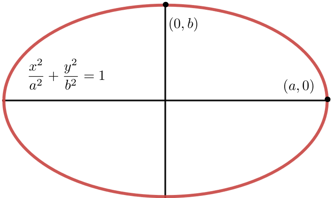
Looking at this graph it appears that the curvature at \((a,0)\) should be greater than at \((0,b)\text{.}\) Use the formula you just derived to verify this.
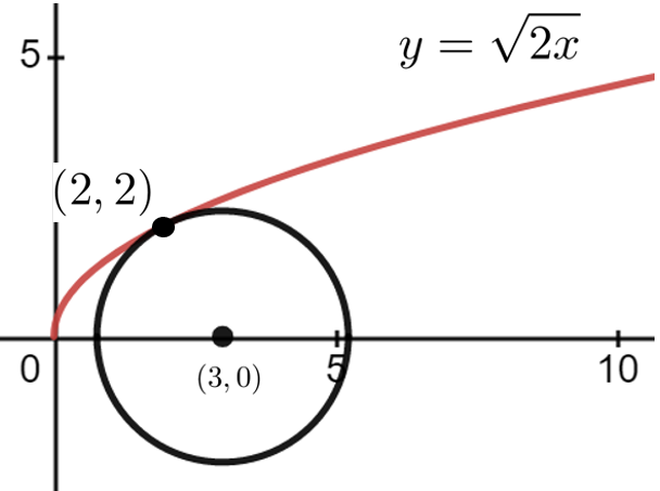
Recall that in Problem 3.5.6 of Section 3.5 we used Descartes’ Method of Normals to find the line tangent to the graph of \(y=\sqrt{2x}\) at the point \((2,2)\) by finding a circle with its center on the \(x\)-axis which touches the graph exactly once, as seen in the sketch below.
Find the equation of the circle which passes through the point \((2,2)\text{,}\) and also has the same slope and curvature as \(y=\sqrt{2x}\) at the point \((2,2)\text{.}\) This is known as the osculating circle, or “kissing circle”.
We observed earlier that if we define curvature using equation (6.19) then the curvature of a straight line will be zero as Oresme said it should be. The converse is also true. Specifically, if \(\abs{\dfdx{\theta}{s}}=\kappa=0\) then \(\theta\) must be a constant and so \(\dfdx{y}{x}=\tan(\theta)\) must also be a constant. (For simplicity we’ll ignore the case where \(\theta=\pm\frac{\pi}{2}\text{.}\))
Assume that \(-\frac{\pi}{2}\lt \theta \lt \frac{\pi}{2}\) and that \(\theta\) is constant. Complete the line of reasoning we began in the previous paragraph to show that
We’ve also shown that the curvature of a circle is also constant. Specifically, it is the reciprocal of the circle’s radius. The converse of this is also true. This can be shown in much the same manner as the straight line (see equation (6.20)) but, naturally, the computations are more complex.
Complete the line of reasoning we began in the previous paragraph to show that \(\dx{y}=\pm\frac1\kappa\sin(\theta)\dx{\theta}\) and \(\dx{x}=\pm\frac1\kappa\cos(\theta)\dx{\theta}\text{.}\)