Differential Calculus: From Practice to Theory

In this section we will state several theorems about limits which we will need in the sections following. The limit concept is very subtle and our understanding of it is still quite intuitive. We are not yet quite prepared to prove these theorems so we will leave these theorems unproven for now. Our immediate goal is simply to understand what they say and learn how to use them. In the next section we will begin using these theorems to show how the limit in Definition 13.2.3 allows us to recapture all of the major results we used in Part I of this text.

In Chapter 17 we will finally discard our intuitive definition of a limit (Definition 12.1.1) and formally define both a limit at infinity (Definition 17.2.19 and Definition 17.2.13) and a limit at a point (Definition 17.3.1). Then we will return to the theorems in this section and (finally) prove rigorously that they are, in fact, true. Until then any result which relies on the theorems in this section should be considered contingent.

But we don’t care if \(\frac{f(x+h)-f(x)}{h}\) is defined at \(h=0\) or not. That is irrelevant to our purpose. So we state explicitly that we do not consider whether \(h=0\text{.}\)

Ok, but why did we insert the word “possibly”? Wouldn’t it be enough to simply say “except at \(a\)”?

We need to say “possibly” because these theorems, like all theorems, are stated with as much generality as possible. For example, consider the function \(f(x)=2x\text{.}\) Had we not included “possibly” in the conditions of our theorems the limit: \(\tlimit{x}{3}{2x}\text{,}\) which is clearly equal to \(6\text{,}\) would have to be considered undefined because \(f(x)=2x\) is defined at \(x=3\text{.}\) This distinction may seem like a very fussy, and unimportant detail right now, but it will be important when we discuss the meaning of continuity in Subsection 14.1.1.

It will be tedious to write (and to read) the phrase “Suppose that \(f(x)\) is defined on some open interval about \(a\) except, possibly, at \(a\) itself” every time we need it so it is customary to say something more like “Suppose \(f(x)\) is defined near \(a\)” instead. Because we are trying to be as precise, and rigorous as possible we will formalize this by redefining the word near.

Notice that this is not what “near” means in ordinary speech. This is one of the things that makes it difficult to read mathematics. We routinely co-opt words from natural languages (like English) and redefine them to fit our needs. In this case our purpose requires that we change the definition of “near” slightly as you’ve seen. Because “near” is a common word and you have a lifetime of experience using it, it can be very difficult to cast off your preconceptions. The familiar definition you learned in childhood will intrude and cause confusion. It is hard to overcome this. Refer back to the definition frequently until you have internalized the mathematical definition.

We have the following theorem.

Since there is no such interval about \(x=0\text{,}\) \(\tlimit{x}{0}{H(x)}\) is undefined.

The following Corollary says that if \(f(x)\) is approaching \(L_f\) and we multiply \(f(x)\) by a number, \(k\text{,}\) then the product \(kf(x)\) approaches \(kL_f\text{.}\) It follows from Theorem 14.1.7 and Theorem 14.1.2.

The concept of continuity is essential to Calculus, but you may have noticed that we have carefully avoided it as much as possible until now. This is because defining continuity is similar to defining the line tangent to a curve (Definition 5.2.4). We need to think carefully about what we want the term continuous to mean, and then craft our definition to capture that meaning. This would have been very difficult to do without a fairly sophisticated understanding of the limit concept.

So stop and think about this for a moment. What do we mean when we say a curve is continuous? A first, intuitive definition usually goes something like this: “A function is continuous if you can draw its graph without lifting your pencil from the paper,” but this is unsatisfactory for a number of reasons. In particular, it is impossible to apply in most cases. Think about it. How often have you seen the entire graph of any function? Usually we just draw the part neat the origin and put arrowheads on both ends of the graph. We need something more precise.

At the end of Example 12.4.31 we remarked that it is only when \(f(x)\) is continuous at \(x=g(a)\) that \(\textcolor{blue}{\tlimit{x}{a}{\textcolor{red}{f(g(x))}}}\) is equal to \(\textcolor{red}{f}\textcolor{blue}{\left(\tlimit{x}{a}{g(x)}\right)}\text{,}\) but we did not discuss the matter any further. It is time for that discussion.

First, notice that when you think closely about the statement “\(f(x)\) is continuous at \(g(a)\)” it appears to be nonsense, because \(g(a)\) is the value of \(f\) at the single value \(g(a)\text{.}\) Does it make sense to you that a curve can be continuous at a single value of its domain? In ordinary usage the concept of continuity requires an interval to be continuous on, doesn’t it?

Since we need the concept of “continuity at a point,” we define it.

If \(f\) is continuous at every point in its domain we’ll just call it a continuous function.

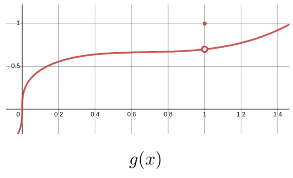
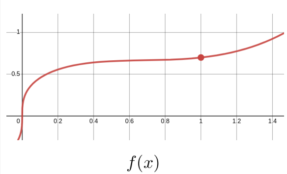
The sketch below shows that Definition 14.1.15 recovers the intuitive notion that a function is continuous if we can draw its graph without lifting pen from page. Both of the functions, \(f(x)\) and \(g(x)\) are identical everywhere except at \(x=1\text{.}\) Clearly, we must lift our pen from the page to draw the graph of \(g(x)\text{,}\) which is discontinuous at \(x=1\text{.}\) But this is not true of the graph of \(f(x)\text{,}\) which is continuous.

Essentially this says that we can interchange the function \(f\) and the “\(\lim\)” symbols if \(f\) is continuous at \(g(a)\text{.}\)

The following lemma is true and the proof will be valid once the limit theorems have been proven in Chapter 17.

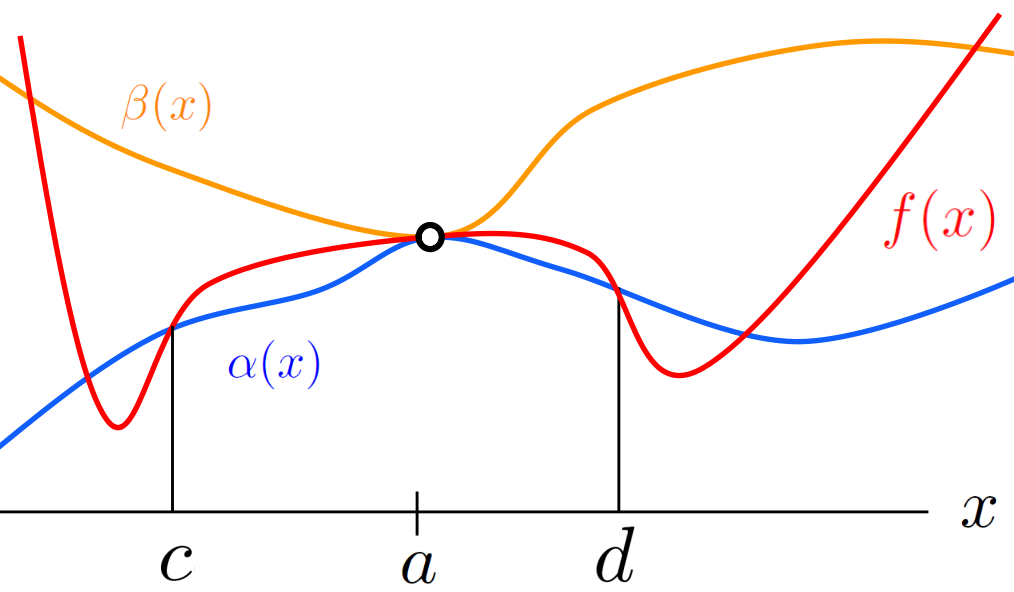
When we were studying horizontal asymptotes in Section 12.2 we encountered Theorem 12.2.2 (the Squeeze Theorem “at” Infinity). But the Squeeze Theorem is also valid if \(x\rightarrow a\text{,}\) where \(a\) is a real number.

Theorem 14.1.19 is illustrated below, but a formal proof will not be given until Chapter 17. Notice that on the interval \((c,d)\) \(f(x)\) is caught between (“squeezed by”) \(\alpha{(x)}\) and \(\beta{(x)}\text{.}\)